Manual de usuario y recetario
Uso completo de la interfaz, diez prácticas reproducibles y una plantilla de bitácora.
Descargar PDF →Versión, DOI, plataformas y arquitectura del software.
Herramientas de escritorio para simulación, análisis visual y generación de figuras reproducibles.
Definiciones vinculadas con resultados numéricos
El diccionario en PDF y las guías web vinculan los conceptos con gráficas obtenidas mediante contratos numéricos explícitos. Esta página identifica los cálculos disponibles, mientras que cada guía desarrolla la configuración, la lectura del resultado y los datos que deben acompañarlo.
Consulta los conceptos de dinámica y caos -> Estudia la ruta universitaria completa en Learning →El diccionario y las guías web vinculan cada definición con una figura reproducible y explican la magnitud calculada por cada diagnóstico.
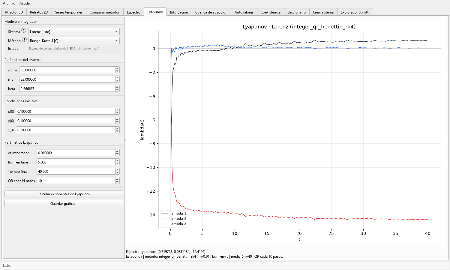
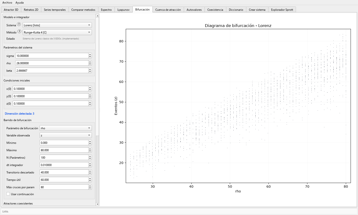
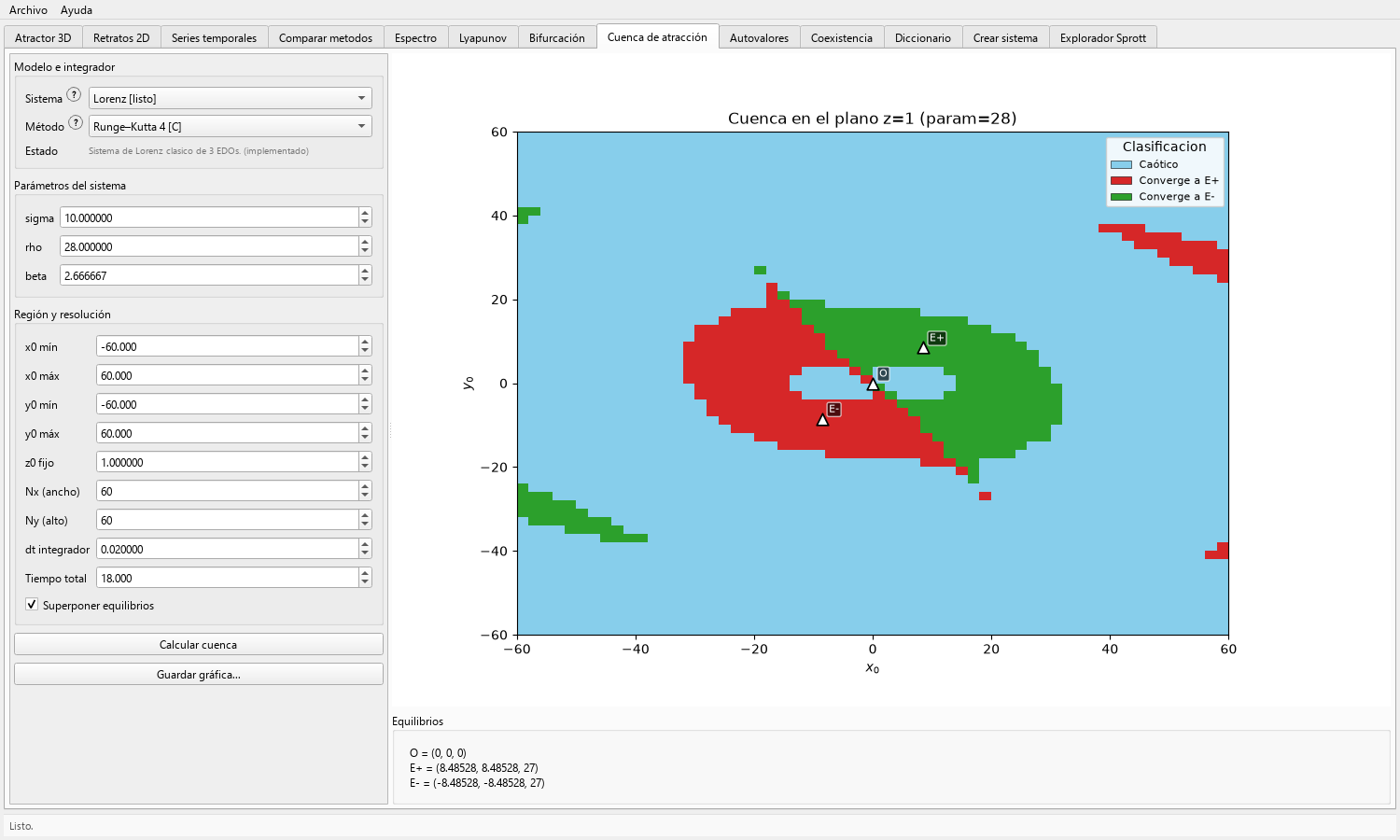
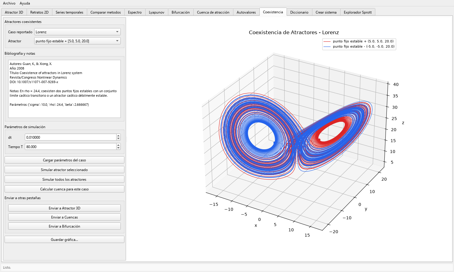
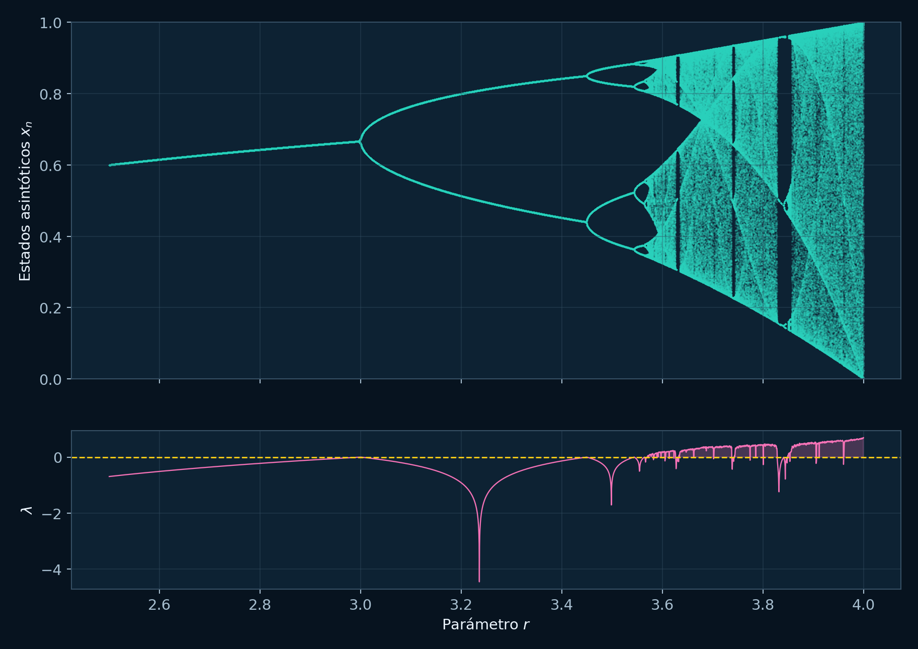
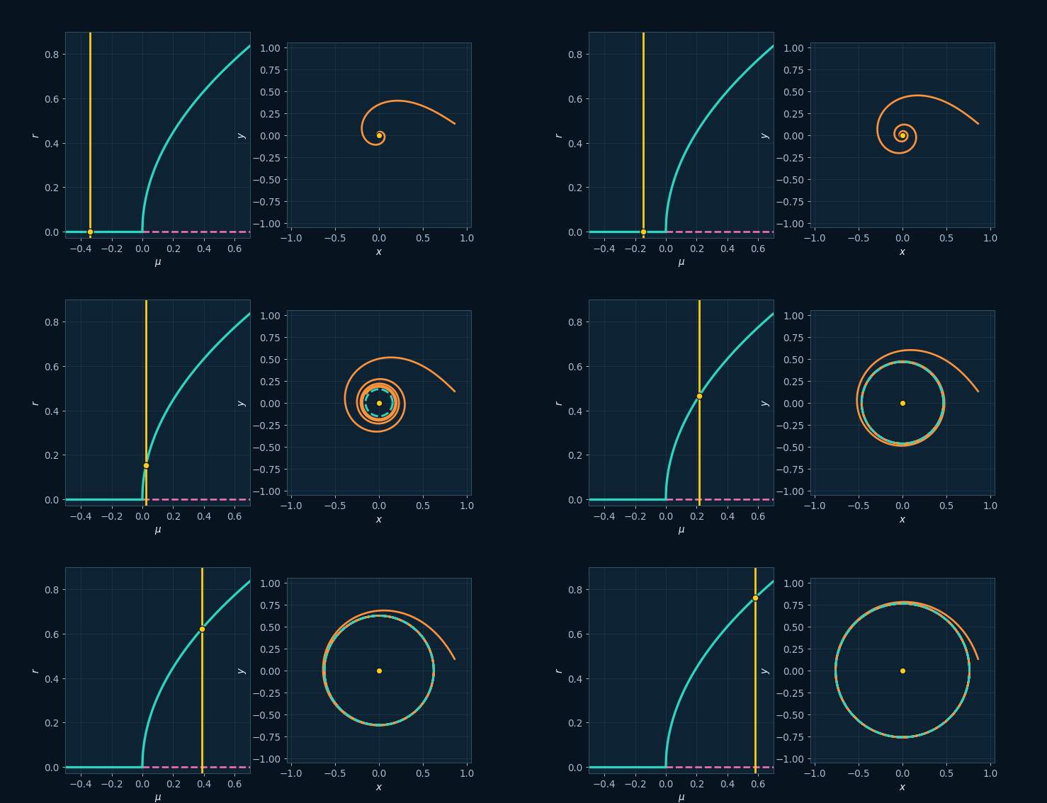
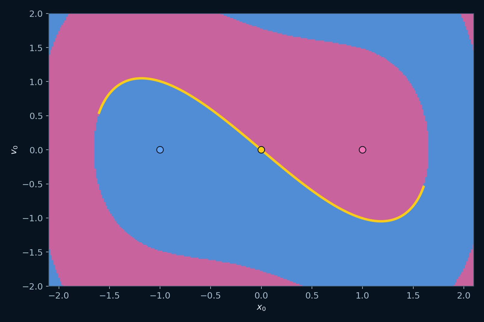
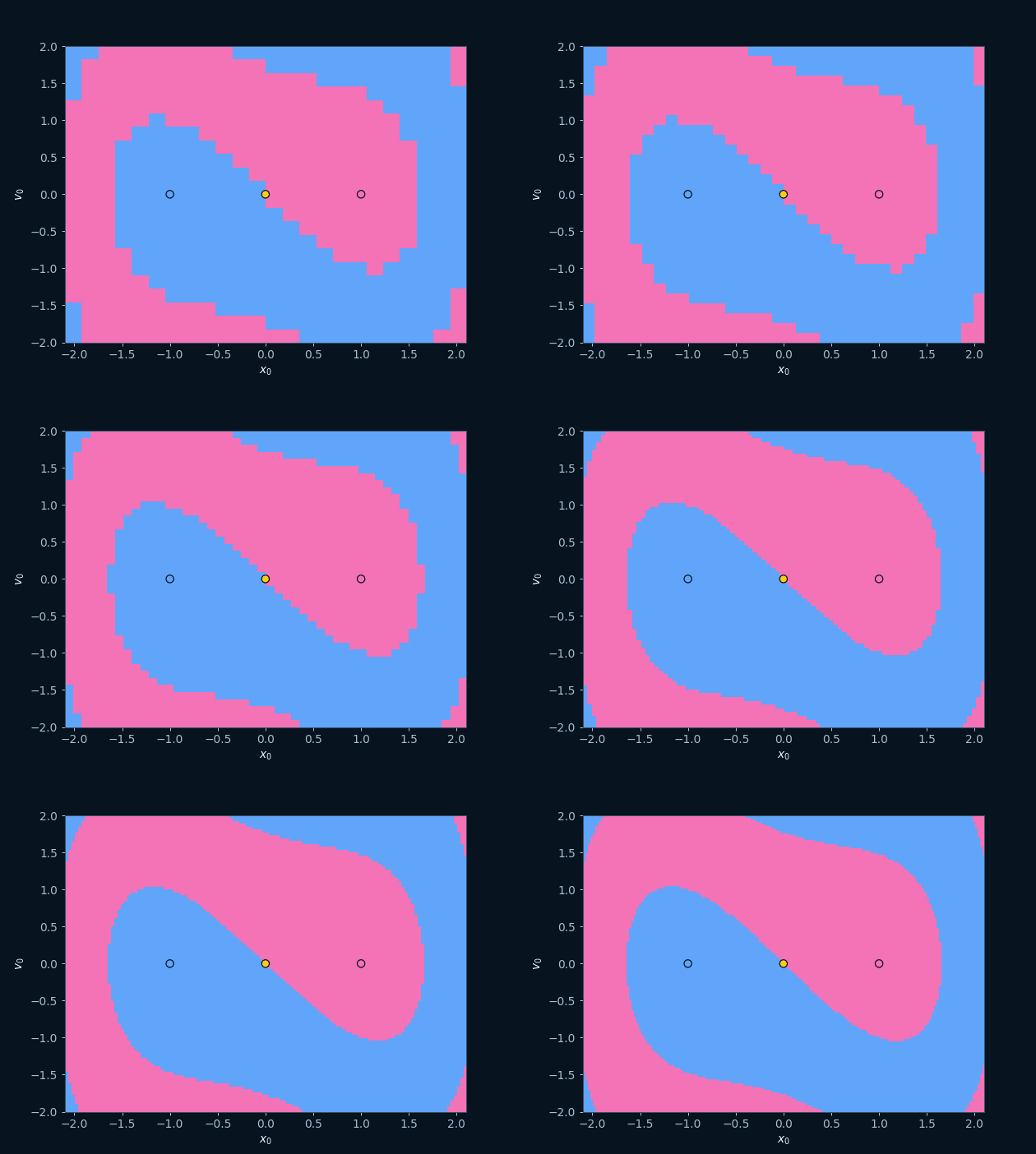
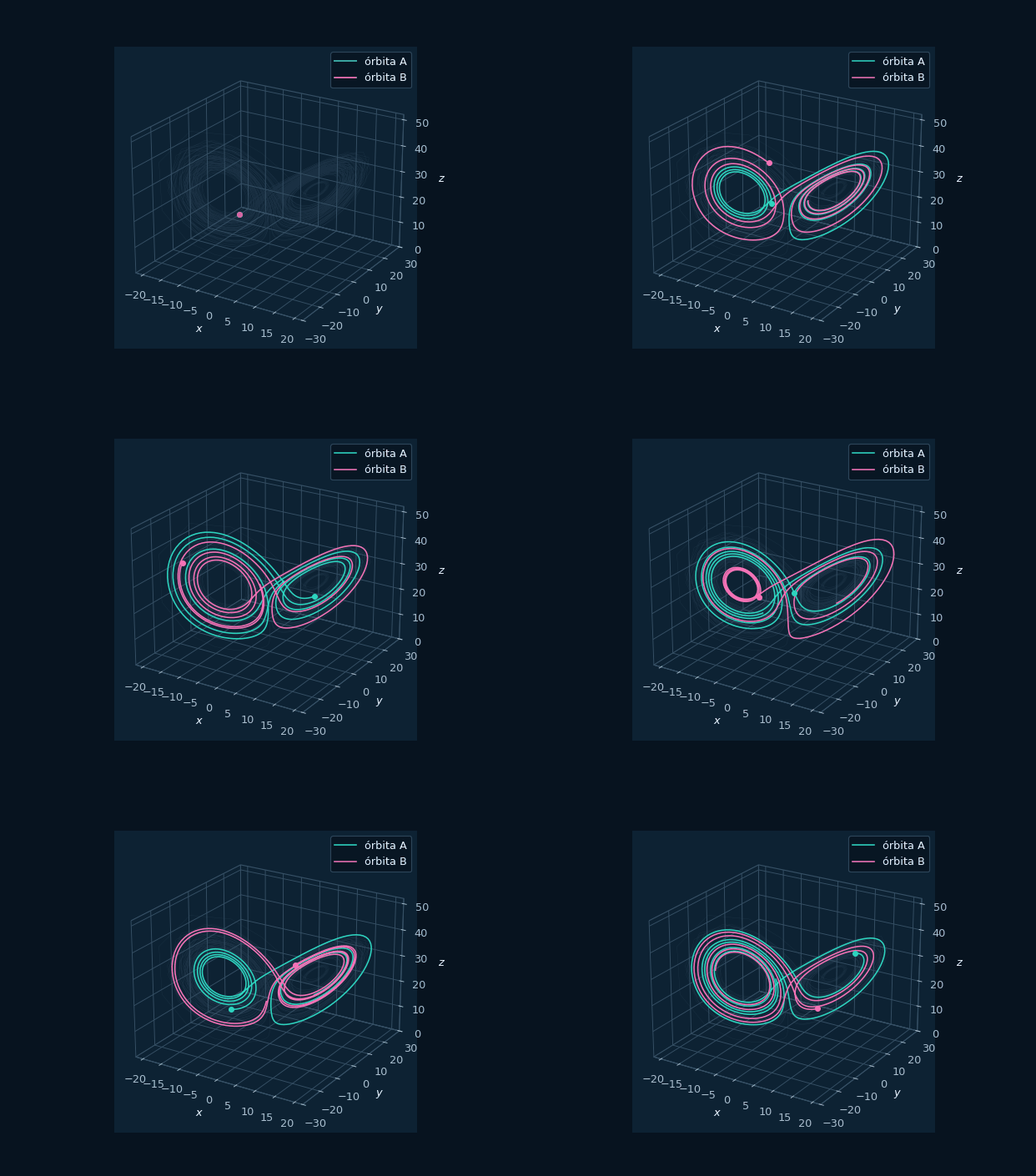
El mapa de cuencas clasifica condiciones iniciales; la vista de coexistencia contrasta destinos; el diagrama de bifurcación recorre un parámetro y la gráfica de Lyapunov estima tasas de separación.
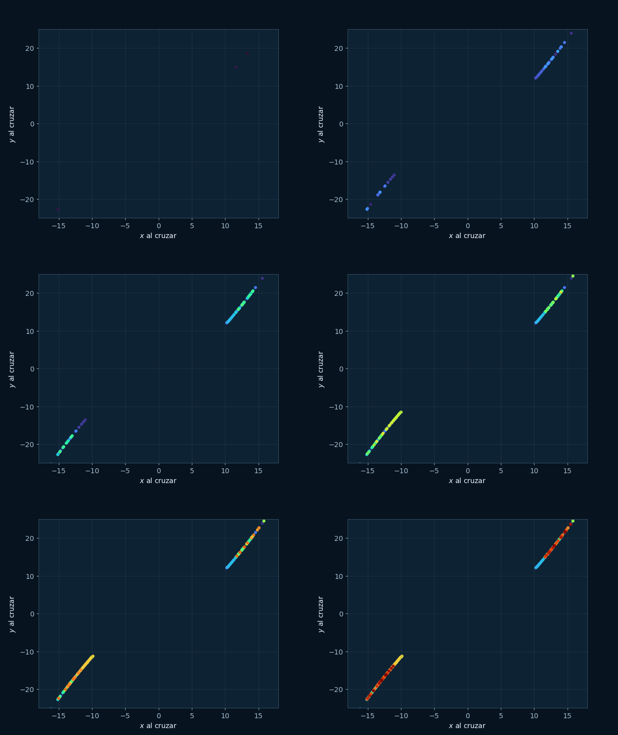
Cada ejemplo registra el sistema, los parámetros, la condición inicial, la proyección y la ventana conservada, de modo que otra ejecución pueda reconstruir la gráfica.
Flujo de exploración de sistemas compactos
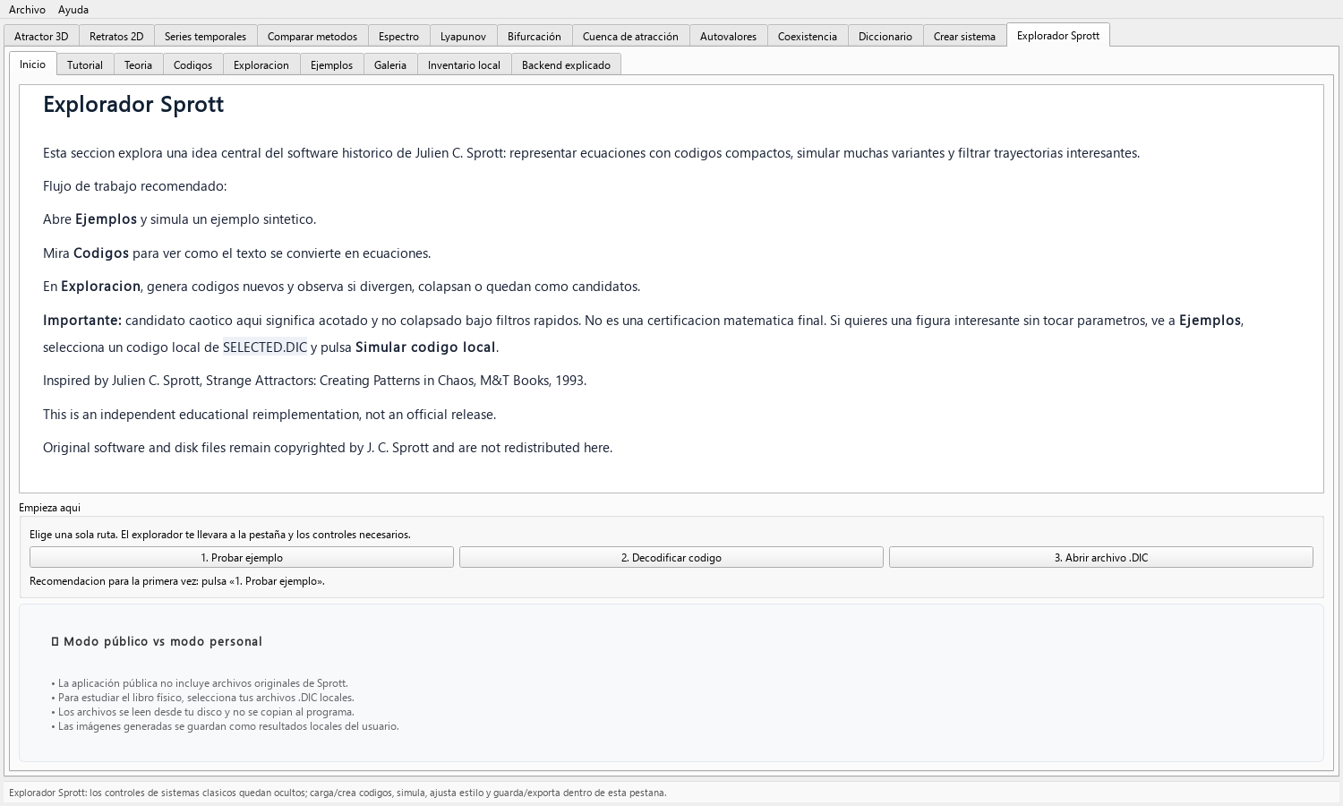
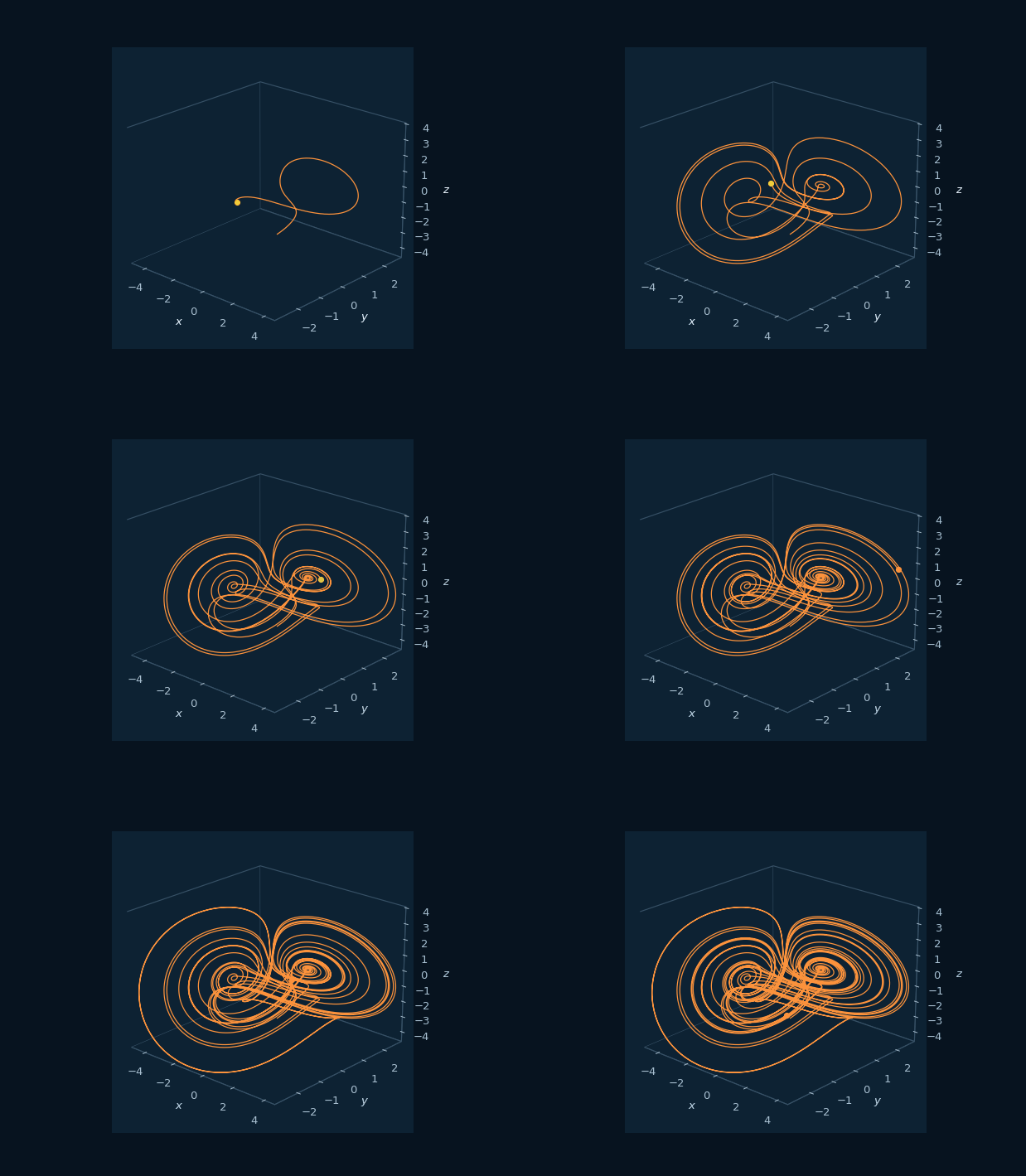
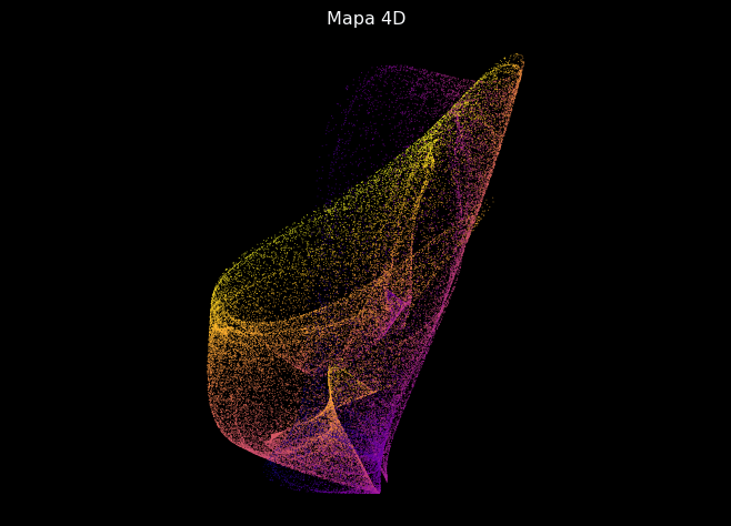
El Explorador Sprott decodifica descripciones compactas inspiradas en el trabajo de J. C. Sprott sobre atractores extraños. A partir de un ejemplo generado, permite ajustar la proyección y los parámetros gráficos para calcular mapas, flujos y representaciones densas del espacio de fases.
Los ejemplos públicos registran su configuración de cálculo. La guía desarrolla la lógica de decodificación, los filtros de búsqueda, las opciones gráficas y el efecto de cada parámetro.
Abre la guía del Explorador Sprott ->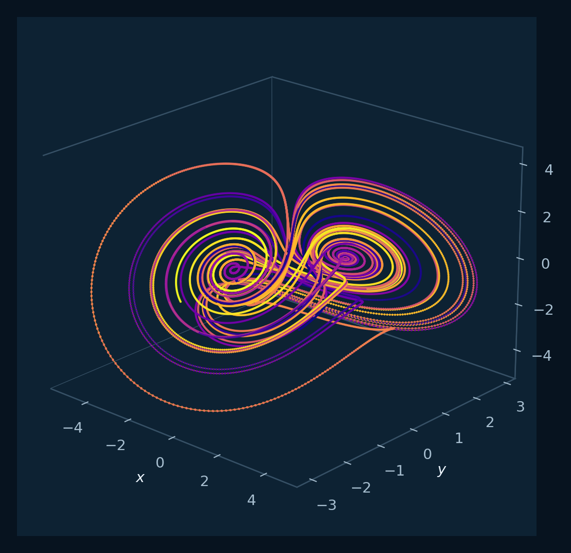
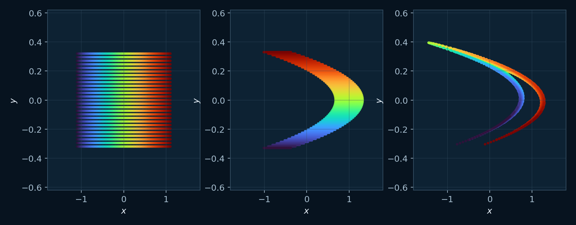
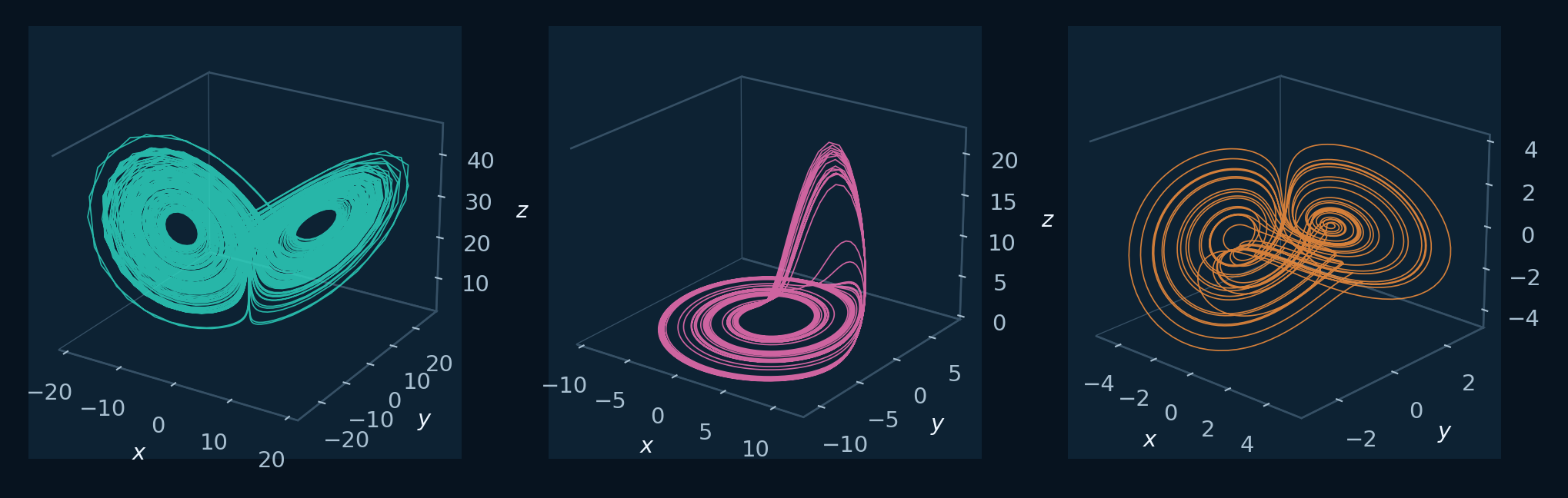
La pregunta determina el modelo, el contrato de integración, el refinamiento y los archivos que documentan la ejecución.
Comienza con la vista o comparación que necesitas: geometría de la trayectoria, evolución temporal, método de integración, espectro, bifurcación, cuenca, coexistencia o estabilidad local.
Usa un sistema registrado para que las ecuaciones, los parámetros, el estado inicial y la escala de integración comiencen en un intervalo conocido.
Usa una malla preliminar, un barrido corto o pocos puntos para verificar el intervalo elegido y estimar el costo del cálculo.
Cambia un valor a la vez: paso temporal, tiempo total, transitorio, intervalo del parámetro, proyección o densidad.
Relaciona la geometría y las series temporales con el método de integración, el espectro, los valores propios, las cuencas, las bifurcaciones o las estimaciones de Lyapunov según la pregunta.
Guarda el sistema, los parámetros, las condiciones iniciales, el método, el paso, el transitorio y la figura o los datos necesarios para reproducir la ejecución.
Las guías describen la instalación, la configuración de cada panel, la generación de figuras, la exportación y los criterios de interpretación científica.
Instale la aplicación de escritorio, ejecute un primer ejemplo del catálogo, reutilice su trayectoria y guarde una figura.
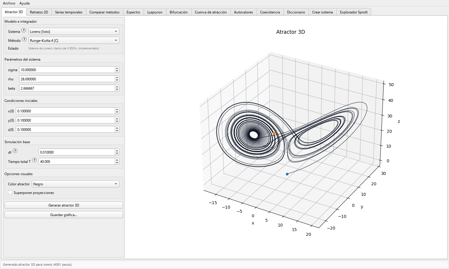
Conozca las 13 pestañas, el flujo compartido de trayectorias, los controles, los mensajes de estado y la función de cada espacio.
Elija entre 38 flujos, mapas, modelos con retardo y modelos especiales; la entrada identifica su implementación y la ejecución numérica aporta la evidencia dinámica.
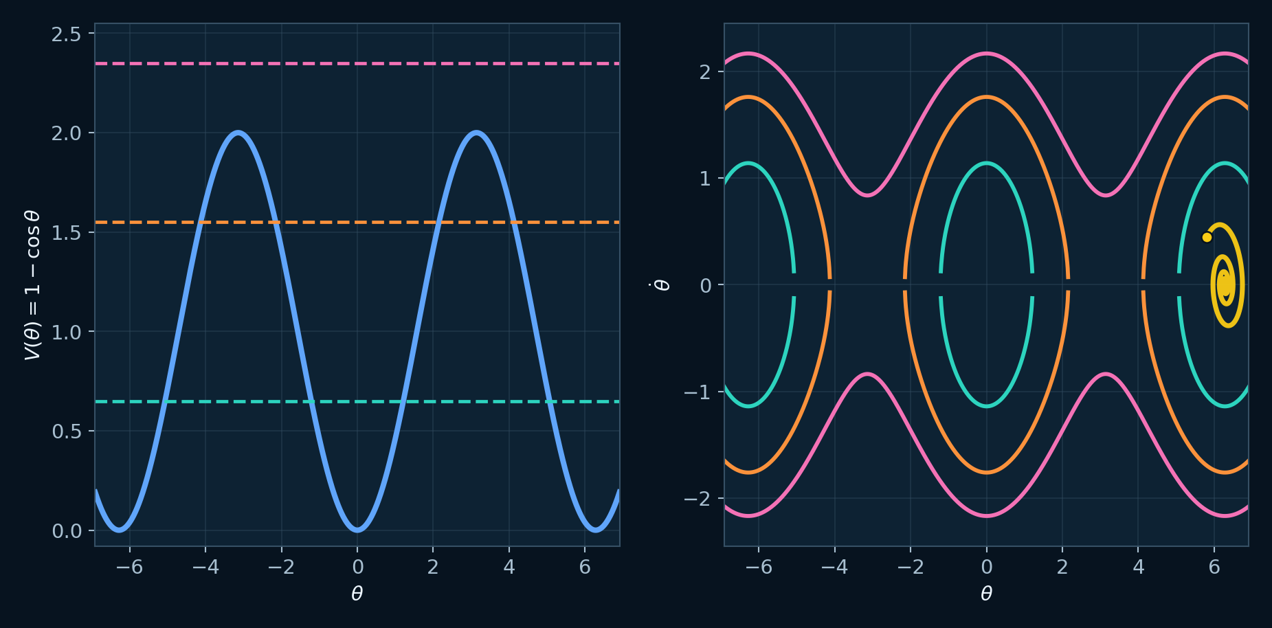
Definiciones y figuras sobre espacio de fases, estabilidad, bifurcaciones, sensibilidad y dinámica caótica.
Diez recetas breves con valores exactos, controles de refinamiento, salidas esperadas y una bitácora común para documentar cada ejecución.
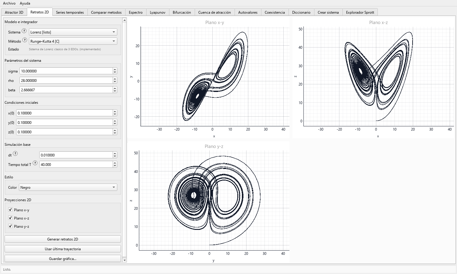
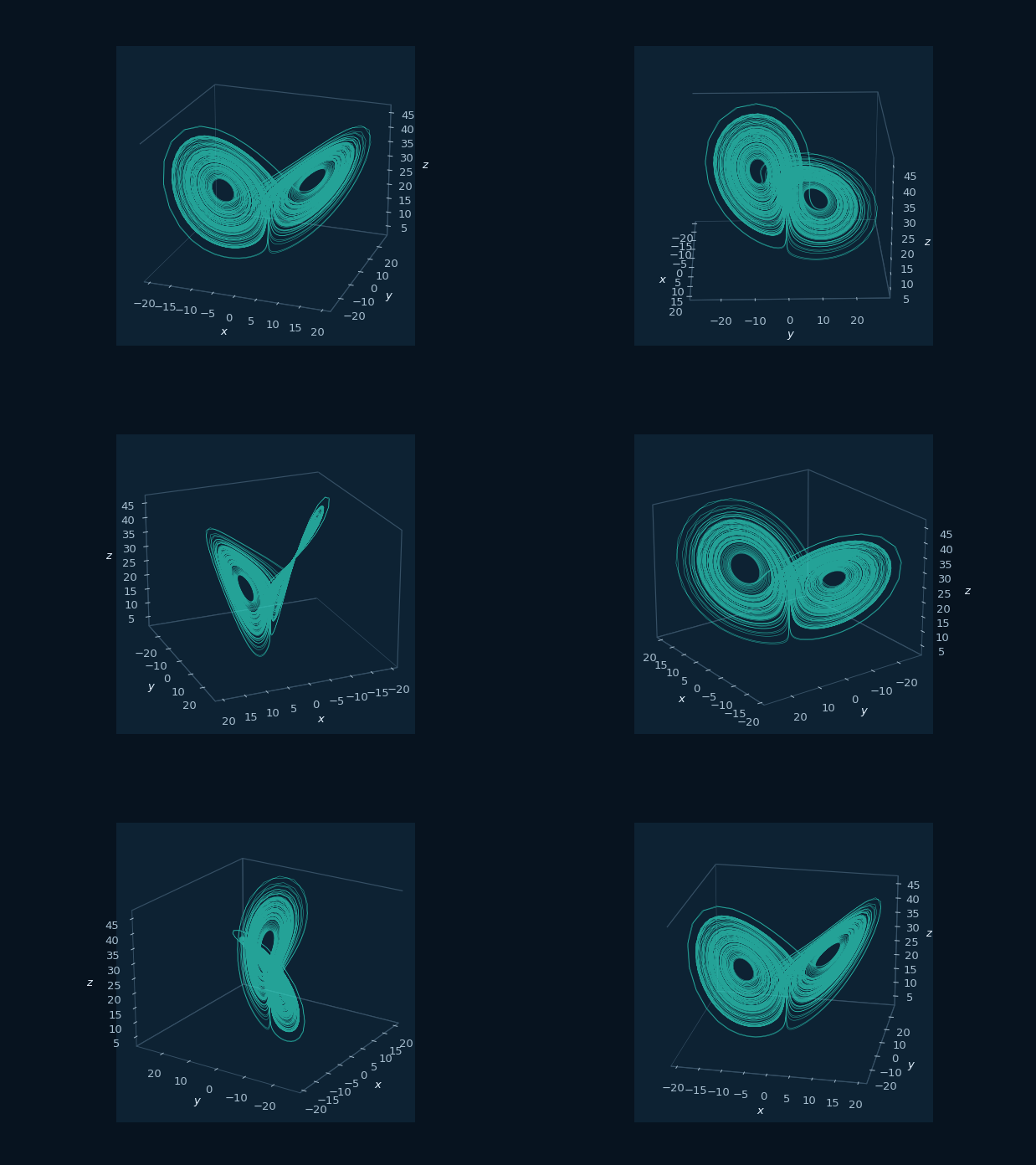
Defina parámetros, ejecute una primera simulación y compare el espacio de fases 3D con retratos proyectados en 2D.
Configure una simulación tridimensional del catálogo, inspeccione sus proyecciones y registre la trayectoria finita representada por la gráfica.
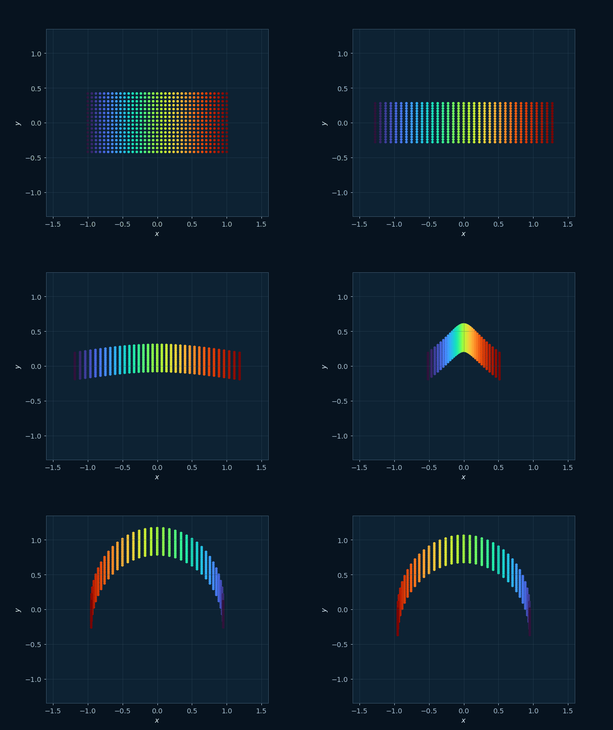
Seleccione pares de variables de estado, reutilice una trayectoria e interprete pliegues, lazos, cruces y artefactos de proyección.
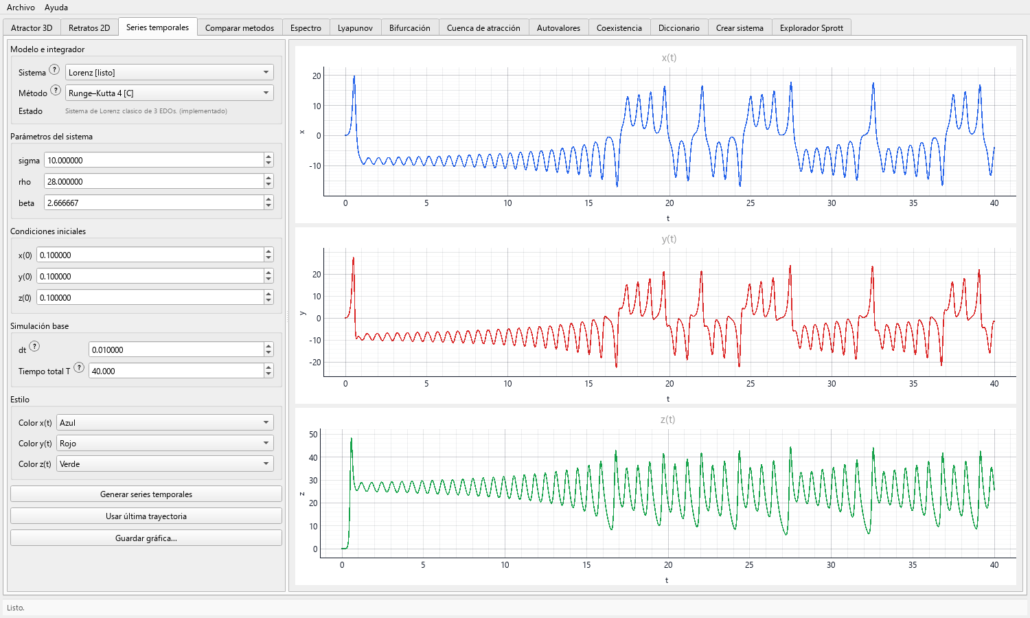
Inspeccione la historia de los estados, transitorios, oscilaciones, ráfagas, deriva y fallas numéricas antes de profundizar el análisis.
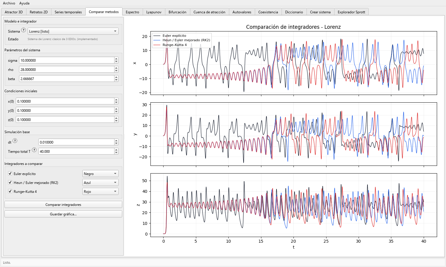
Compare Euler, Heun y RK4 bajo el mismo contrato numérico y realice un estudio práctico del tamaño de paso.
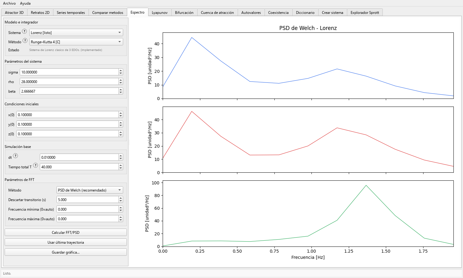
Elija la PSD de Welch o un espectro de amplitud, descarte transitorios, defina límites de frecuencia e interprete correctamente las unidades.
Ejemplo concentrado en generar e interpretar el espectro de amplitud del sistema de Lorenz.
Visualice el crecimiento de perturbaciones e interprete estimaciones de exponentes a tiempo finito atendiendo su convergencia.
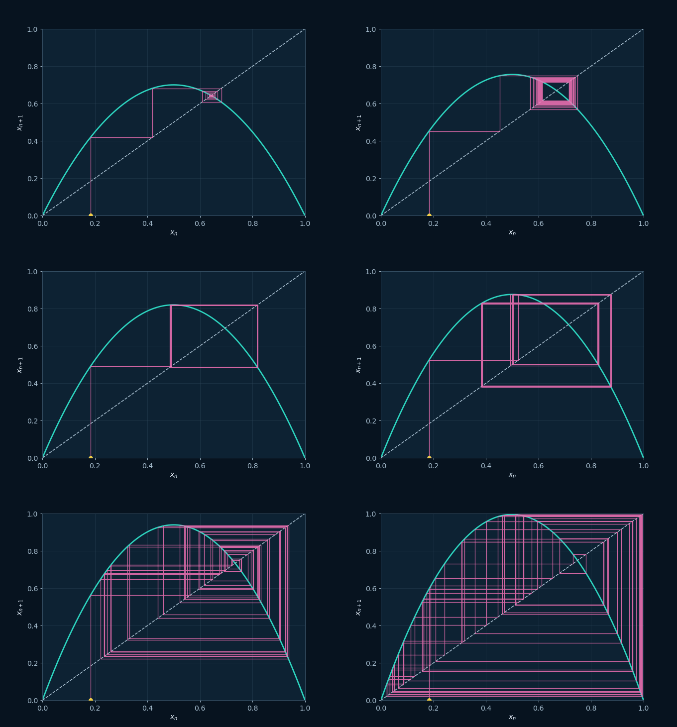
Configure barridos de parámetros, puntos retenidos, secciones de Poincaré y ejemplos de Hopf.
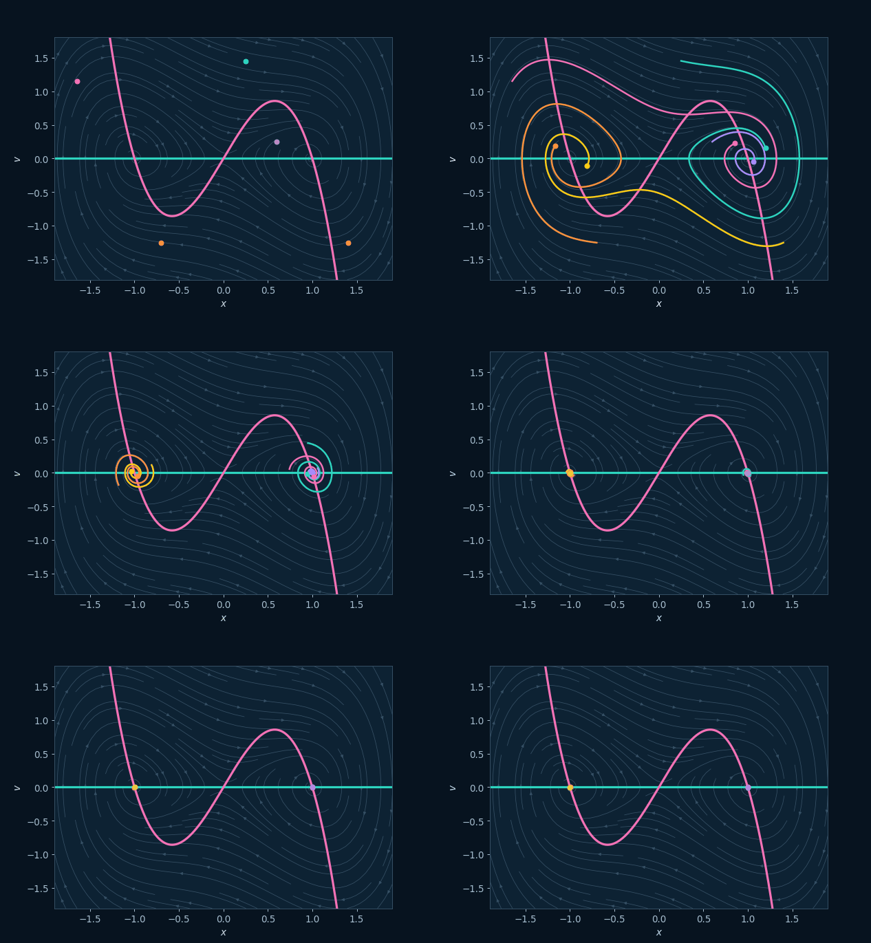
Interprete mapas de cuencas a resolución finita y trayectorias representativas iniciadas en distintas regiones.
Compare casos de multiestabilidad registrados con parámetros fijos y condiciones iniciales distintas.
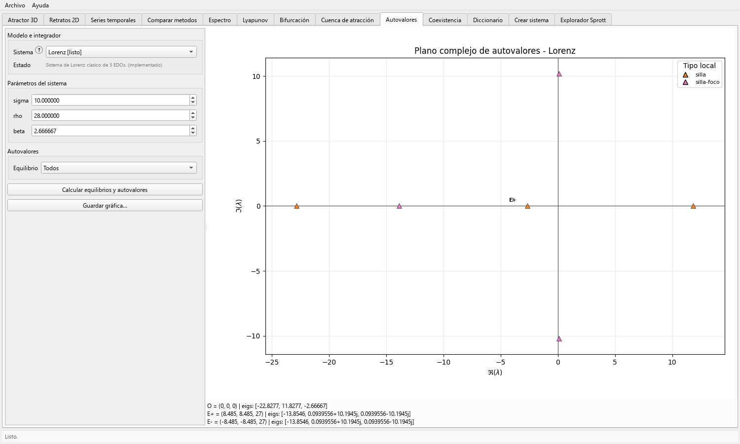
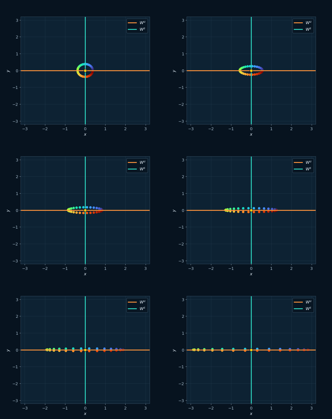
Calcule equilibrios de EDO compatibles, inspeccione los valores propios del jacobiano y comunique responsablemente la estabilidad lineal local.
Comprenda los códigos, la decodificación, la búsqueda, los filtros, los ajustes visuales y los diccionarios locales del usuario.
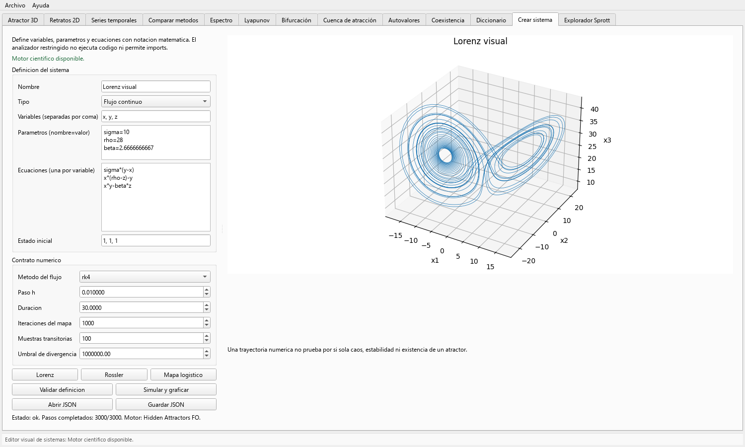
Defina, valide, simule, importe y exporte un flujo o mapa con el editor de expresiones.
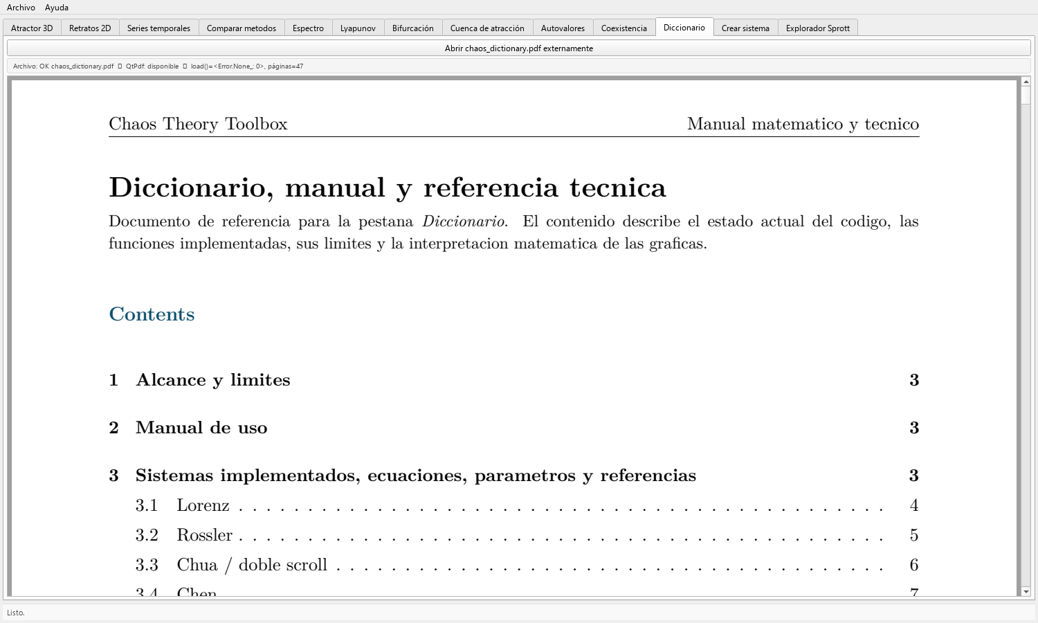
Use el diccionario integrado como apoyo didáctico y conecte las definiciones con gráficas y experimentos numéricos.
Guarde figuras y definiciones, registre el contrato numérico y prepare un conjunto de resultados que otra persona pueda auditar.
Planifique estudios paramétricos, matrices comparativas y exploraciones de multiestabilidad que conserven la evidencia.
Indique las magnitudes mostradas por las gráficas y los cálculos finitos, y adjunte los estudios de convergencia o el análisis formal exigidos por la afirmación.
Biblioteca en PDF
Tres documentos complementan las guías web: consulta el curso para la teoría, el recetario para trabajar con la interfaz y el manual Sprott para seguir la decodificación paso a paso.
Uso completo de la interfaz, diez prácticas reproducibles y una plantilla de bitácora.
Descargar PDF →Gramática de códigos, desarrollo algebraico, métodos numéricos, filtros y contratos de exportación.
Descargar PDF →Curso progresivo de sistemas dinámicos y caos con ecuaciones, interpretación gráfica, problemas y lecturas.
Descargar PDF →Espacios de trabajo actuales de la interfaz y ejemplos representativos de atractores, bifurcaciones, secciones de Poincaré, cuencas, coexistencia, figuras de Lyapunov y gráficas generadas por el Explorador Sprott.
Si utilizas este software en investigaciones, tesis o actividades académicas, cita la versión archivada en OSF.
Maria Fernanda Moreno Lopez. Fyskode Chaotic Systems Toolbox, version 0.1.0. 10.17605/OSF.IO/GQMJR.