Manual pedagógico · nivel inicial a intermedio

Curso esencial de sistemas dinámicos y caos

Ruta pedagógica desde estado, órbitas y estabilidad hasta bifurcaciones, caos, integración numérica e interpretación responsable de las gráficas de Toolbox Chaos.

Abrir el curso completo en Fyskode Learning

Pregunta y resultado

Cálculo que realizará

Construir una base teórica suficiente para formular, simular e interpretar experimentos de sistemas dinámicos continuos y discretos con Toolbox Chaos.

Pestaña de la interfaz

Diccionario y pestañas científicas asociadas a cada módulo

Configuración y cálculo

Secuencia de controles

Siga los módulos en orden: regla de evolución, espacio de estados, estabilidad, bifurcaciones, caos, métodos numéricos y lectura de diagnósticos.
En cada módulo, derive primero la ecuación breve y después reproduzca el ejemplo indicado en la interfaz.
Conserve ecuaciones, parámetros, estado inicial, método, resolución, horizonte y transitorio junto a cada gráfica.
Resuelva los ejercicios antes de consultar las pistas y repita al menos una ejecución con resolución refinada.
Complete la formación con el curso enlazado y las lecturas anotadas al final de cada bloque.

Registro

Datos obtenidos

Un cuaderno que conecte definiciones y ecuaciones con series temporales, retratos de fase, bifurcaciones, cuencas, espectros y estimaciones de Lyapunov.
Conclusiones delimitadas por la resolución y el horizonte del cálculo, con una comparación de refinamiento y archivos suficientes para repetirlo.

Lectura científica

Criterios de interpretación

Una órbita, una serie temporal y un espectro son representaciones distintas del mismo experimento; cada una contesta una pregunta diferente.

La estabilidad local procede del jacobiano cerca de un equilibrio, mientras que el comportamiento global requiere trayectorias, secciones, cuencas y diagnósticos de largo plazo.

Archivos

Registro del experimento

Guarde las figuras con un pie que identifique sistema, parámetros, variable o proyección, método, paso, horizonte y transitorio.
Añada un archivo de texto o JSON con el estado inicial, controles del diagnóstico, resultado del refinamiento y límites de la interpretación.

Aplicaciones

Preguntas que admite el cálculo

Curso introductorio de licenciatura sobre ecuaciones diferenciales no lineales y mapas iterados.
Preparación de prácticas de laboratorio con comparación entre predicción analítica y cálculo numérico.
Lectura crítica de gráficas científicas de dinámica no lineal.

Alcance

Condiciones de la evidencia

Una figura irregular abre una hipótesis de trabajo; sostenga sensibilidad, mezcla, atracción o persistencia con los diagnósticos y controles apropiados.
Los exponentes y espectros de tiempo finito dependen del transitorio, la resolución y la ventana observada.
La concordancia numérica se comprueba con refinamiento; una demostración formal requiere sus hipótesis y su argumento correspondiente.

Ruta de estudio

Orden de conceptos y diagnósticos

La primera vuelta ocupa ocho sesiones. En las sesiones 1 y 2 se aprende a leer la regla de evolución y el espacio de estados; en las sesiones 3 y 4 se estudian equilibrio, linealización y bifurcaciones; en las sesiones 5 y 6 se introducen sensibilidad, exponentes de Lyapunov, secciones y espectros; en las sesiones 7 y 8 se comparan integradores y se redacta una interpretación reproducible. Una segunda vuelta debe transformar cada ejemplo guiado: cambie un parámetro, anticipe el efecto, ejecute el cálculo y explique cualquier diferencia entre la predicción y la gráfica.

El ritmo recomendado es definición, derivación breve, simulación, lectura de la figura, ejercicio y refinamiento. La ecuación se estudia junto con su protocolo numérico. Si una trayectoria se calcula con paso h, la comparación con h/2 conserva el mismo tiempo total; si se estudia un mapa, se conserva el mismo número de iteraciones útiles después del transitorio.

Módulo 1 · Regla, estado y tiempo

Regla de evolución y espacio de estados

Un sistema dinámico combina un conjunto de estados con una regla que determina su evolución. En tiempo continuo, el estado $x(t)\in\mathbb R^D$ satisface una ecuación diferencial autónoma. En tiempo discreto, la regla avanza por iteraciones enteras:

\dot x=f(x;\mu),\qquad x(0)=x_0,\qquad\text{o bien}\qquad x_{n+1}=F(x_n;\mu)

El vector μ reúne parámetros. Una solución continua define un flujo $\varphi^t(x_0)$ ; un mapa define la sucesión $x_n=F^n(x_0)$ . El modelo es determinista cuando el mismo estado y los mismos parámetros producen la misma evolución, aunque una sensibilidad intensa haga difícil predecir a largo plazo.

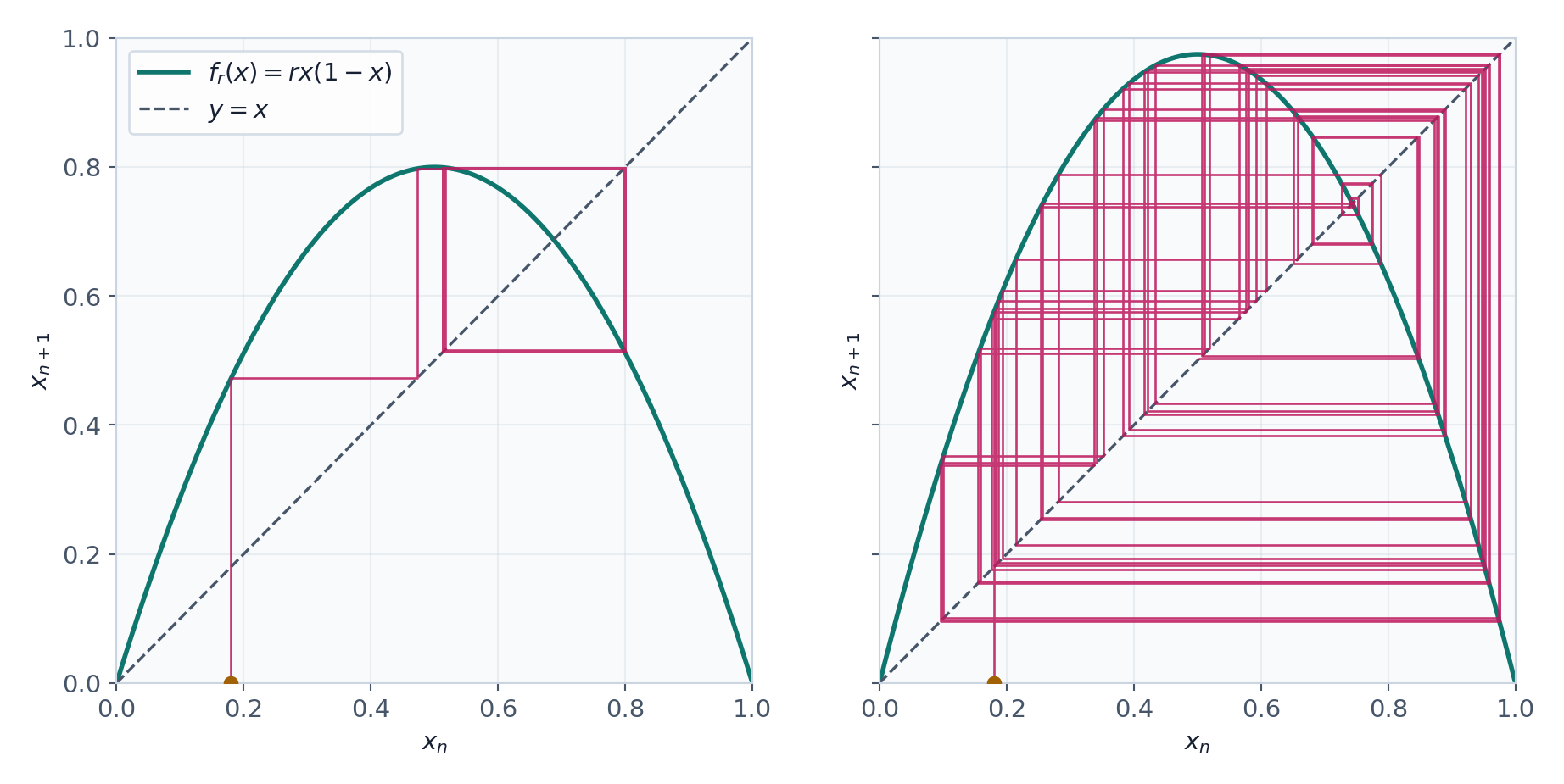
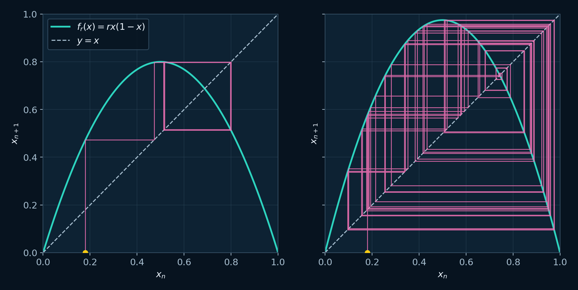
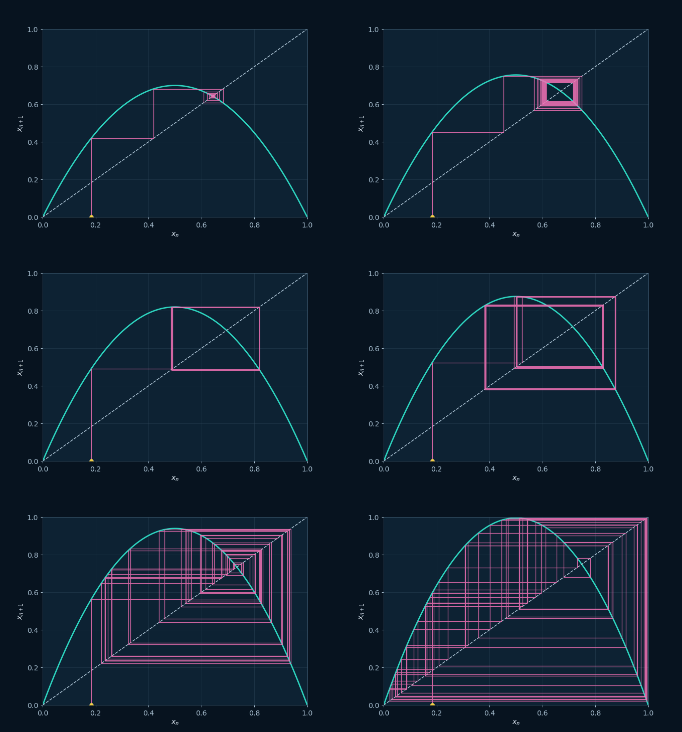
La primera práctica usa el mapa logístico $x_{n+1}=r x_n(1-x_n)$ . Con r=2.8 y x0=0.2, la sucesión se aproxima a $x^*=1-1/r$ . Con r=3.2 aparece una oscilación estable de periodo dos. La pestaña de bifurcación permite ver cómo esos destinos cambian al recorrer r.

Iteraciones del mapa logístico construidas con una telaraña geométrica — La diagonal devuelve cada salida como la entrada siguiente. Active la secuencia y observe si los escalones se acercan a un punto, alternan entre varios niveles o dejan de cerrar; esa geometría traduce la regla xₙ₊₁=F(xₙ) en una evolución visible.

Ejercicio 1. Calcule a mano las primeras cinco iteraciones para r=2.8. Después derive los dos puntos fijos resolviendo F(x)=x y compruebe cuál atrae a x0=0.2. Pista: estudie

|F'(x^*)|

Módulo 2 · Geometría de las soluciones

Órbitas, retratos de fase e invariancia

La trayectoria temporal enumera el estado conforme transcurre el tiempo; la órbita es el conjunto geométrico recorrido en el espacio de fases. Un retrato 2D dibuja, por ejemplo, y contra x y elimina la lectura explícita del tiempo. Los cruces aparentes de una proyección se interpretan con el estado completo. En un flujo autónomo con unicidad, las órbitas mantienen trayectorias diferenciadas en el espacio de fases completo.

Un conjunto S es invariante si una órbita que empieza en S permanece en S. Un conjunto atractor, en el sentido operativo de una práctica numérica, debe ser invariante y recibir trayectorias de una vecindad; una nube acotada observada durante un tiempo finito sólo sugiere qué conjunto estudiar. La cuenca reúne los inicios que alcanzan el mismo destino bajo el protocolo definido.

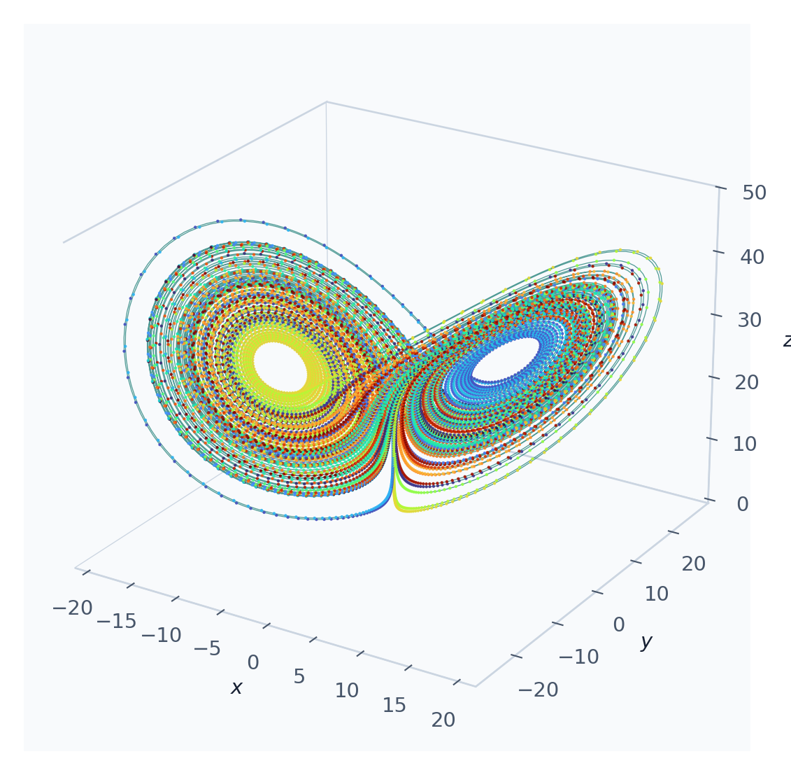
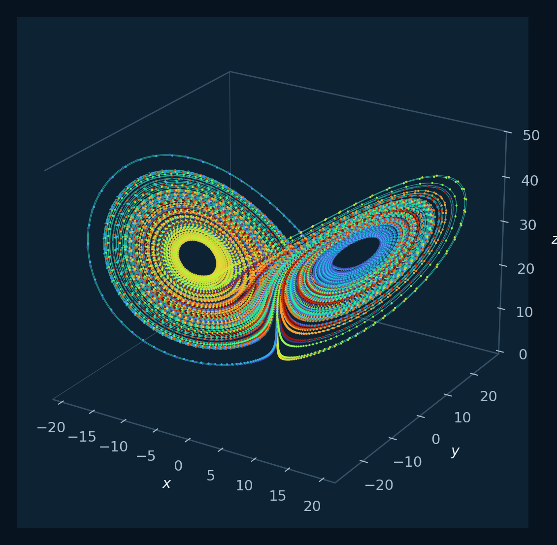
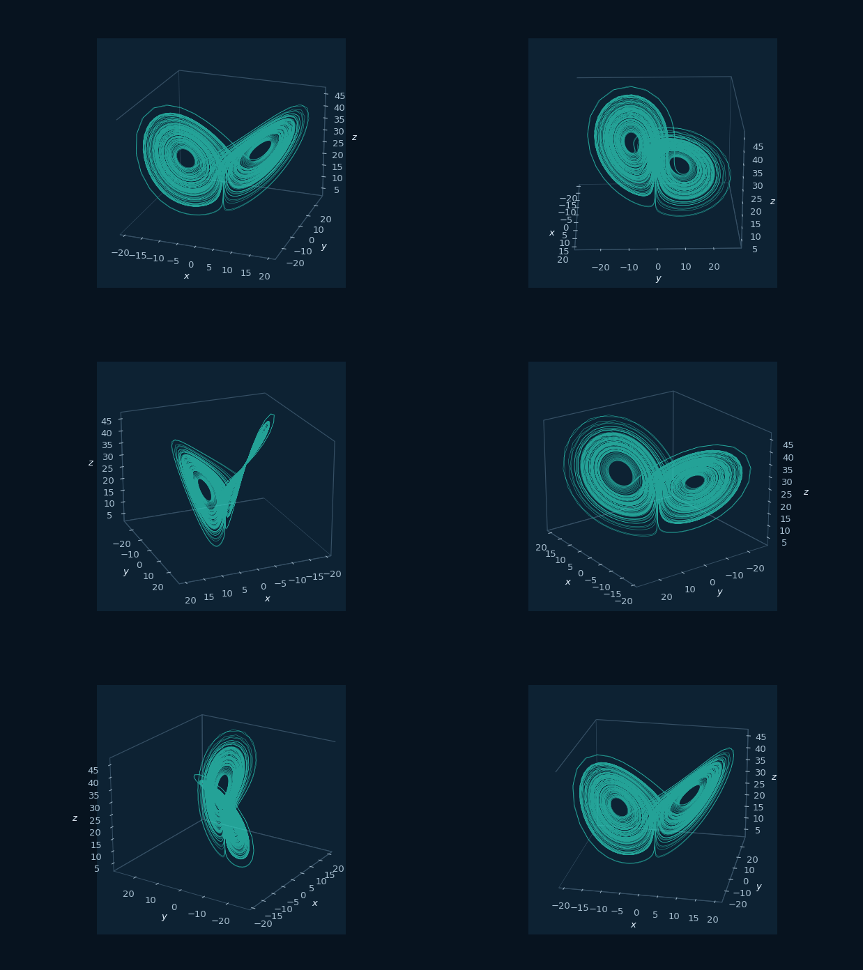
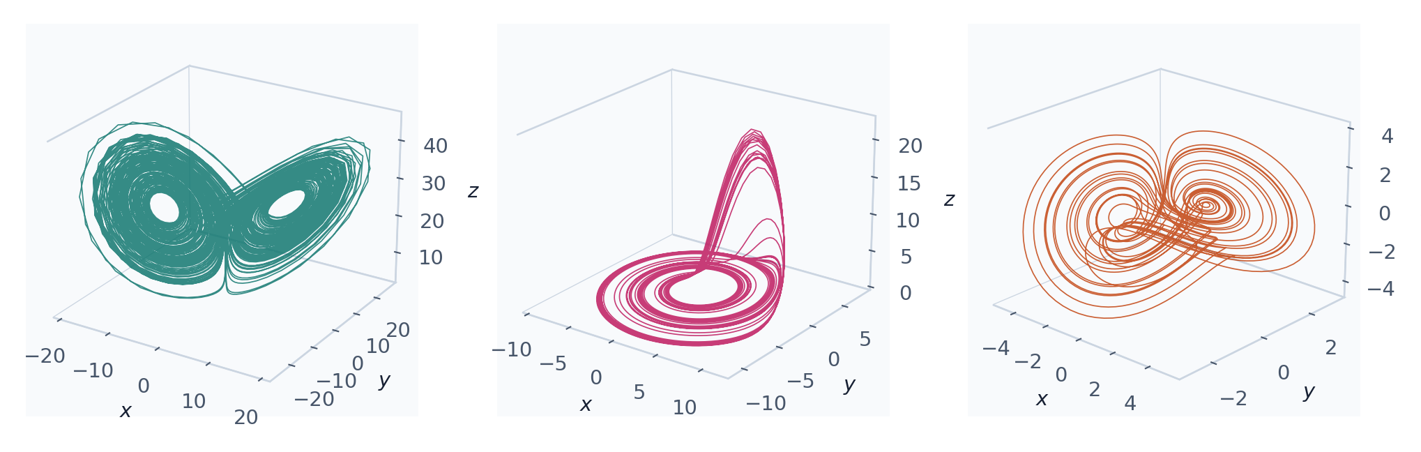
Trayectoria tridimensional del sistema de Lorenz en Toolbox Chaos — La rotación cambia la proyección desde la que se observa la misma órbita. Busque qué cruces aparentes se separan al girar y recupere el orden temporal mediante la serie o la animación del recorrido.

En Toolbox Chaos seleccione Lorenz con σ=10, ρ=28, β=8/3, x0=(0.1,0.1,0.1), RK4, dt=0.01 y T=40. Compare la vista 3D con los planos xy, xz y yz. El doble lóbulo persiste, pero cada proyección oculta una coordenada y puede superponer segmentos separados.

Ejercicio 2. Exporte las tres proyecciones de Lorenz y marque una región que parece cruzarse. Use la coordenada omitida o la vista 3D para decidir si el cruce es real. Repita con dt=0.005 y T=40.

Módulo 3 · Equilibrio y estabilidad local

Linealizar cerca de un estado estacionario

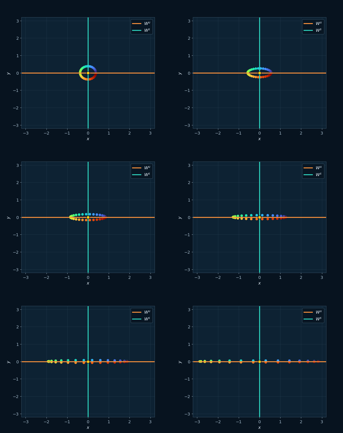
Un equilibrio x* de un flujo satisface f(x*)=0. Cerca de él, escribimos x=x*+ξ y retenemos la primera variación. El jacobiano $J_{ij}=\partial f_i/\partial x_j$ gobierna la aproximación lineal:

\dot\xi=J(x^*)\xi+O(\|\xi\|^2),\qquad \xi(t)\approx e^{Jt}\xi(0)

Si todos los valores propios de J tienen parte real negativa, el equilibrio es localmente asintóticamente estable. Una parte real positiva produce una dirección inestable. En un mapa se reemplaza la parte real por el módulo: la estabilidad lineal exige que todos los multiplicadores de DF(x*) tengan módulo menor que uno.

Para Lorenz, el origen siempre es equilibrio y los otros dos aparecen cuando ρ>1:

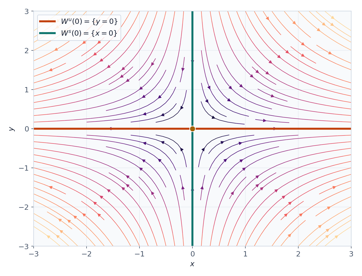
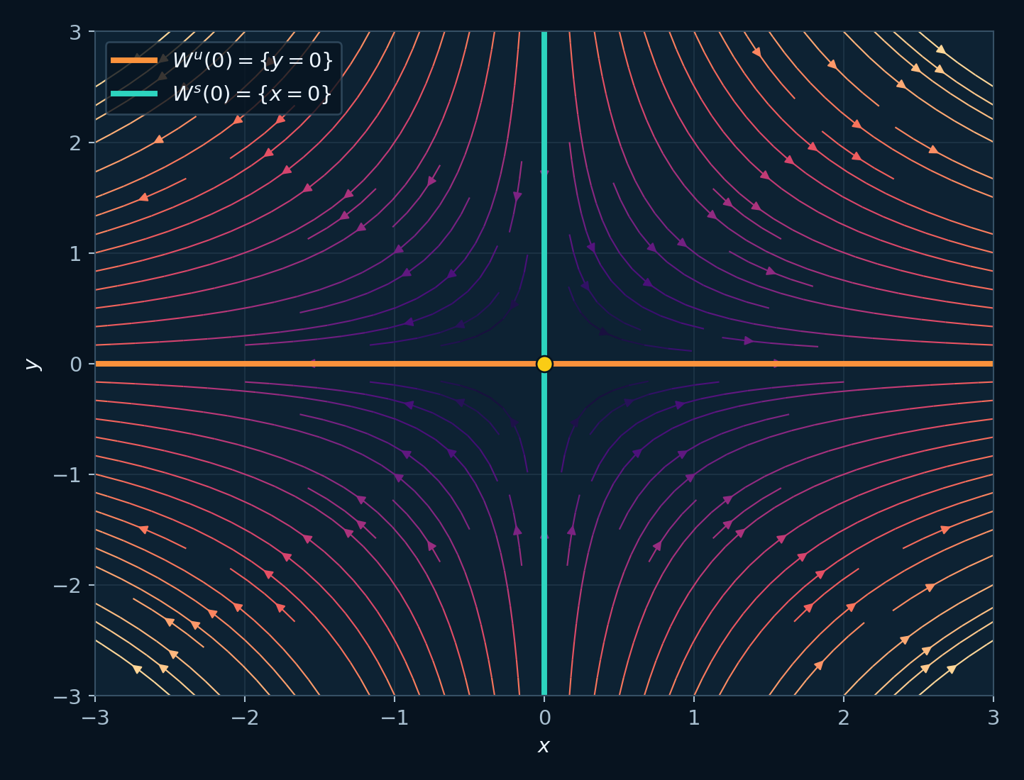
C_{\pm}=\left(\pm\sqrt{\beta(\rho-1)},\ \pm\sqrt{\beta(\rho-1)},\ \rho-1\right)

Abra Equilibrios y valores propios, calcule los tres puntos para ρ=24.4 y compare la clasificación local con trayectorias que empiezan cerca. La linealización describe un entorno del punto; la geometría lejana requiere el análisis global correspondiente.

Direcciones estable e inestable alrededor de un punto silla — Las trayectorias se acercan por la dirección estable y se alejan por la inestable. La animación permite relacionar los signos de los valores propios con el movimiento local; las regiones alejadas requieren el análisis global correspondiente.

Ejercicio 3. Para

\dot x=x-x^3

, obtenga los equilibrios, evalúe f′ y clasifíquelos. Dibuje después la recta de fases y explique por qué la clasificación coincide con las flechas.

Módulo 4 · Parámetros y bifurcaciones

Cuando cambia la organización cualitativa

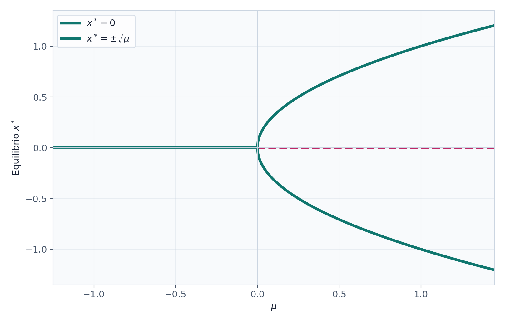
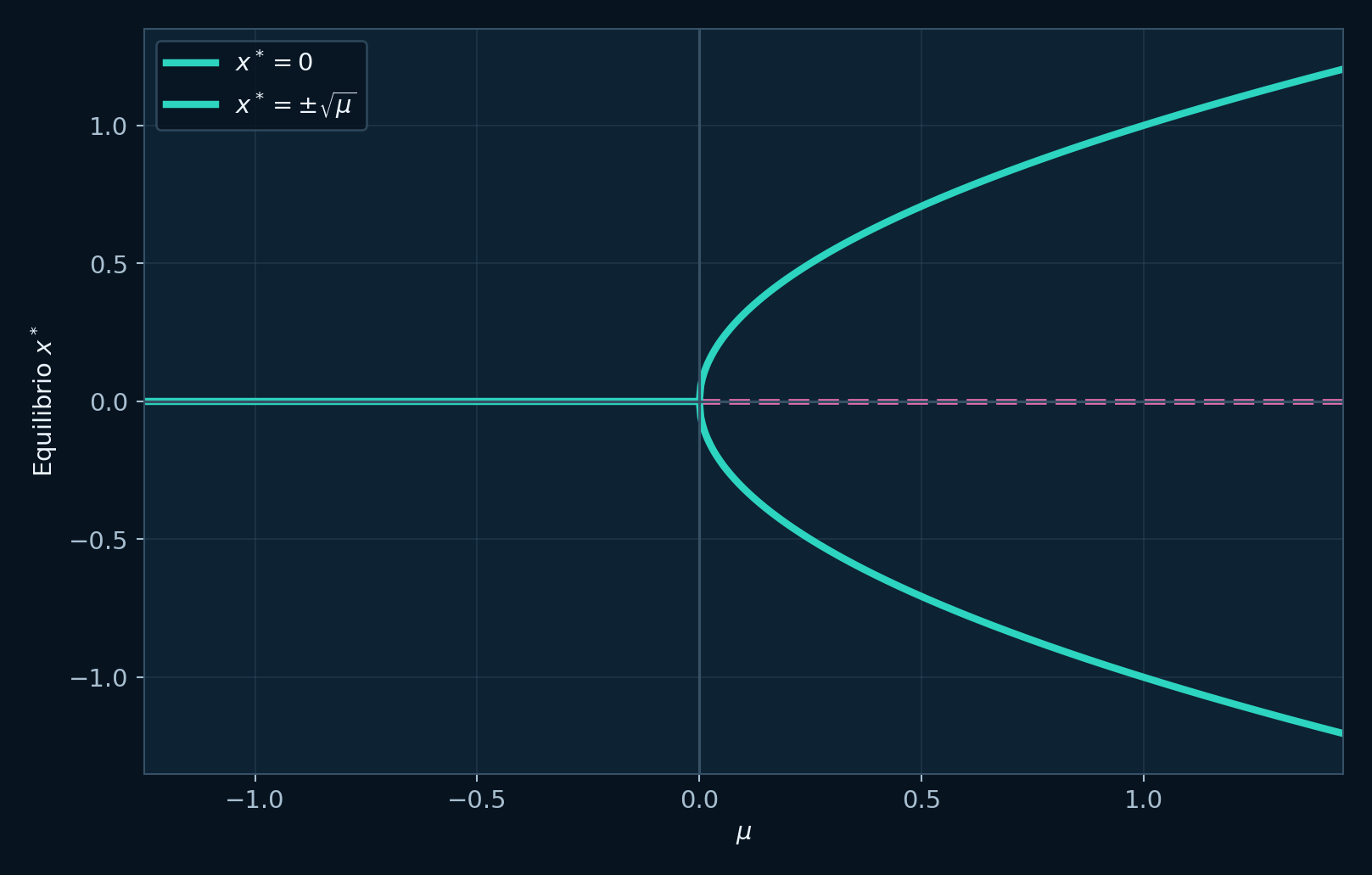
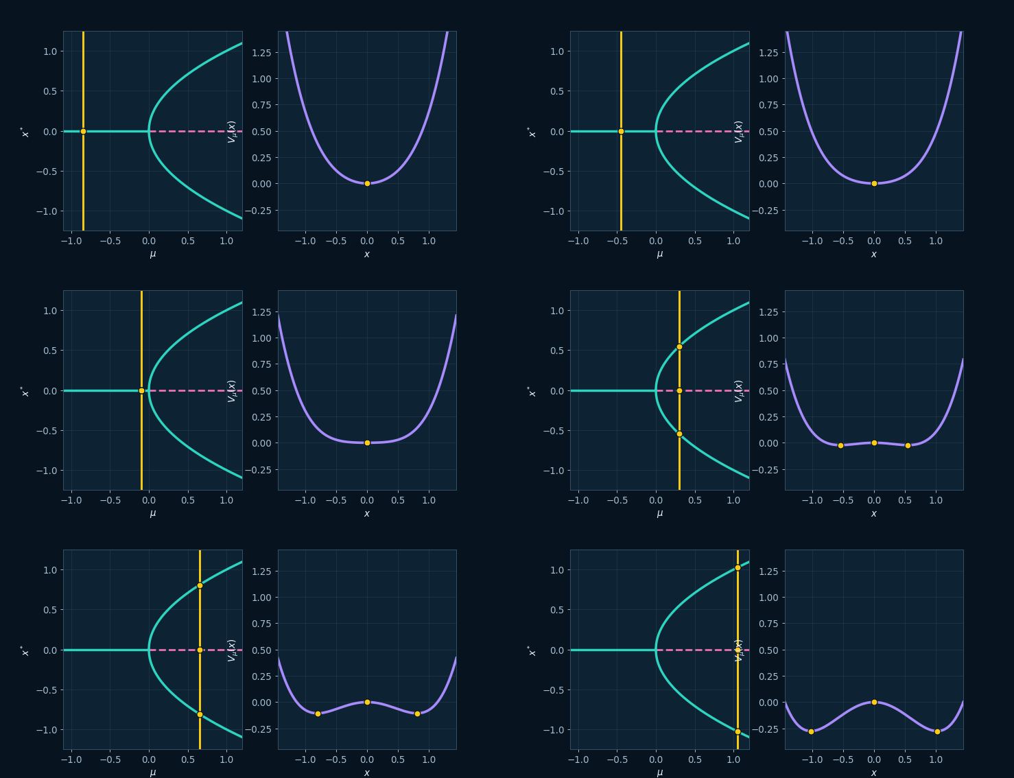
Una bifurcación ocurre cuando variar un parámetro modifica la cantidad, estabilidad o tipo de objetos invariantes. La forma normal silla-nodo $\dot x=\mu-x^2$ crea dos equilibrios para μ>0. La transcrítica $\dot x=\mu x-x^2$ intercambia estabilidad entre ramas. La pitchfork supercrítica $\dot x=\mu x-x^3$ rompe una simetría y crea dos ramas estables.

En dos dimensiones, una bifurcación de Hopf se asocia con un par complejo conjugado que cruza el eje imaginario. La forma normal radial

\dot r=\mu r-r^3,\qquad \dot\theta=\omega

muestra el mecanismo: para μ<0 el origen atrae; para μ>0 aparece un ciclo de radio √μ. El nacimiento local de una oscilación requiere diagnósticos adicionales para clasificar caos. En mapas, el cruce de un multiplicador por −1 produce duplicación de periodo; el diagrama logístico organiza una cascada de estas duplicaciones.

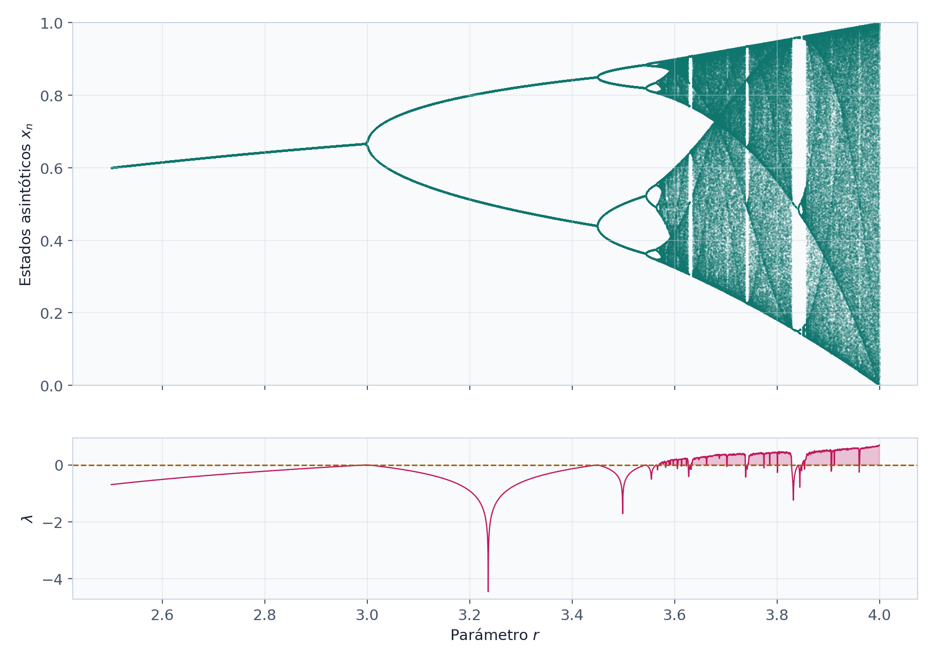
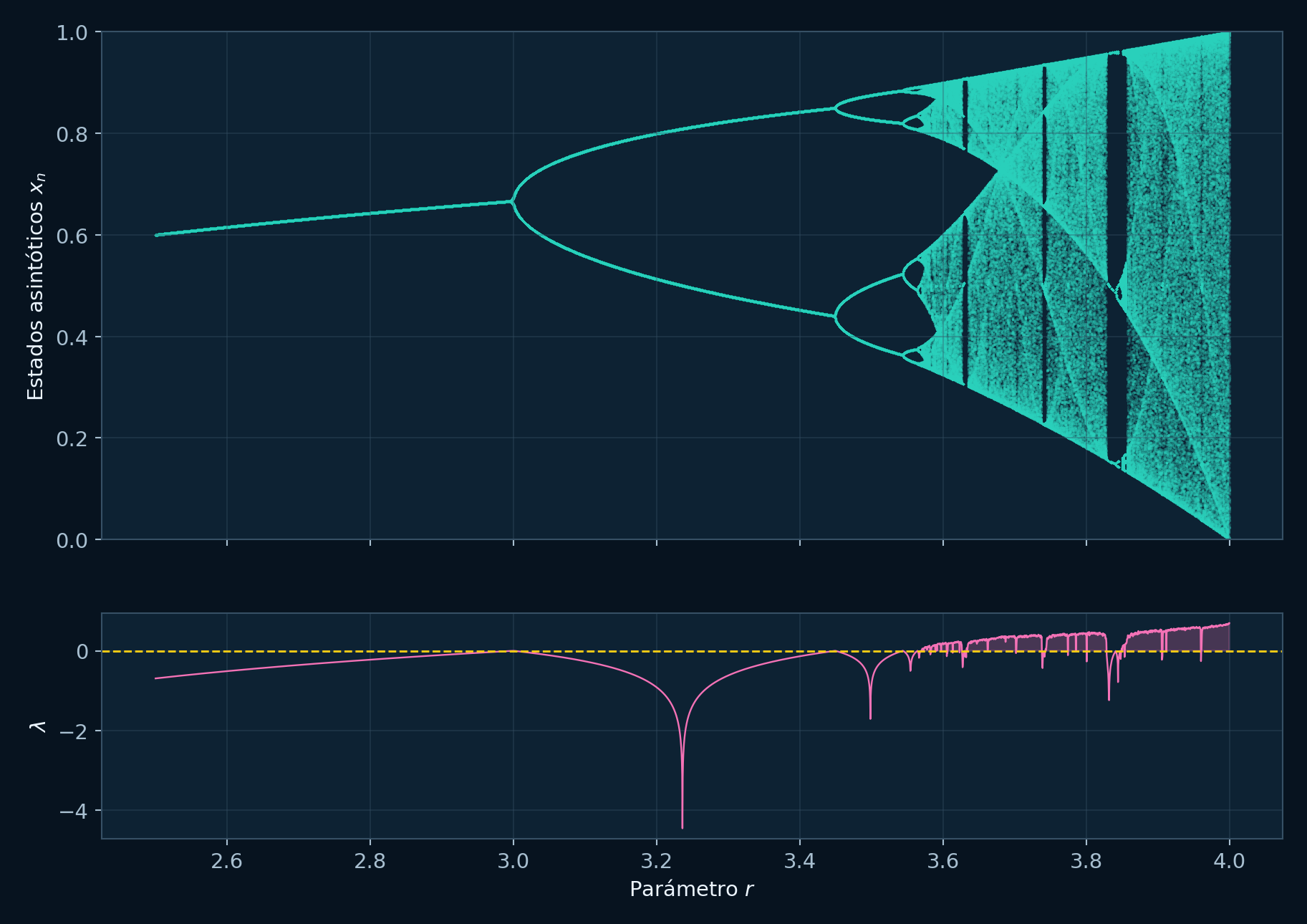
Ramas de equilibrio de una bifurcación de horquilla supercrítica — Siga la rama central al variar μ: su cambio de estabilidad coincide con el nacimiento de dos ramas simétricas. La figura representa equilibrios analíticos; para visualizar ramas inestables se requiere un procedimiento que cubra esas soluciones.

Diagrama de bifurcación del mapa logístico — Cada columna conserva estados posteriores al transitorio para un valor de r. Una, dos o cuatro alturas indican ciclos de esos periodos; una banda densa exige volver a una serie individual y comprobar resolución, transitorio y sensibilidad.

En la pestaña Bifurcación, barre r de 2.5 a 4 con 350 valores, elimina 600 iteraciones y conserva 500. Vuelve a calcular con 700 valores y 1000 iteraciones de transitorio. Una rama estable se ve como un solo nivel; un ciclo de periodo k forma k niveles; una banda densa exige diagnósticos adicionales.

Ejercicio 4. Derive los equilibrios y la estabilidad de la forma pitchfork. Después identifique en un diagrama qué parte corresponde a equilibrio inestable y explique por qué un barrido que sólo dibuja estados alcanzados puede omitirla.

Módulo 5 · Sensibilidad y exponentes

Sensibilidad de trayectorias cercanas

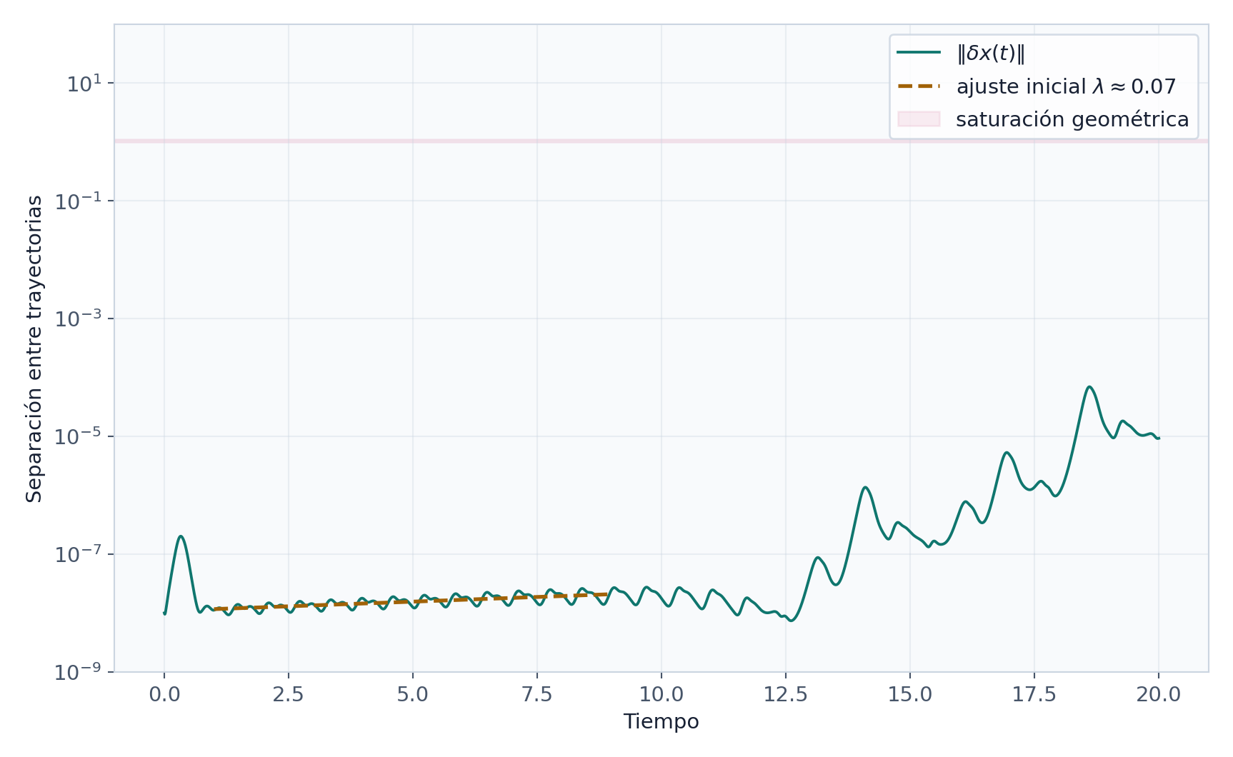
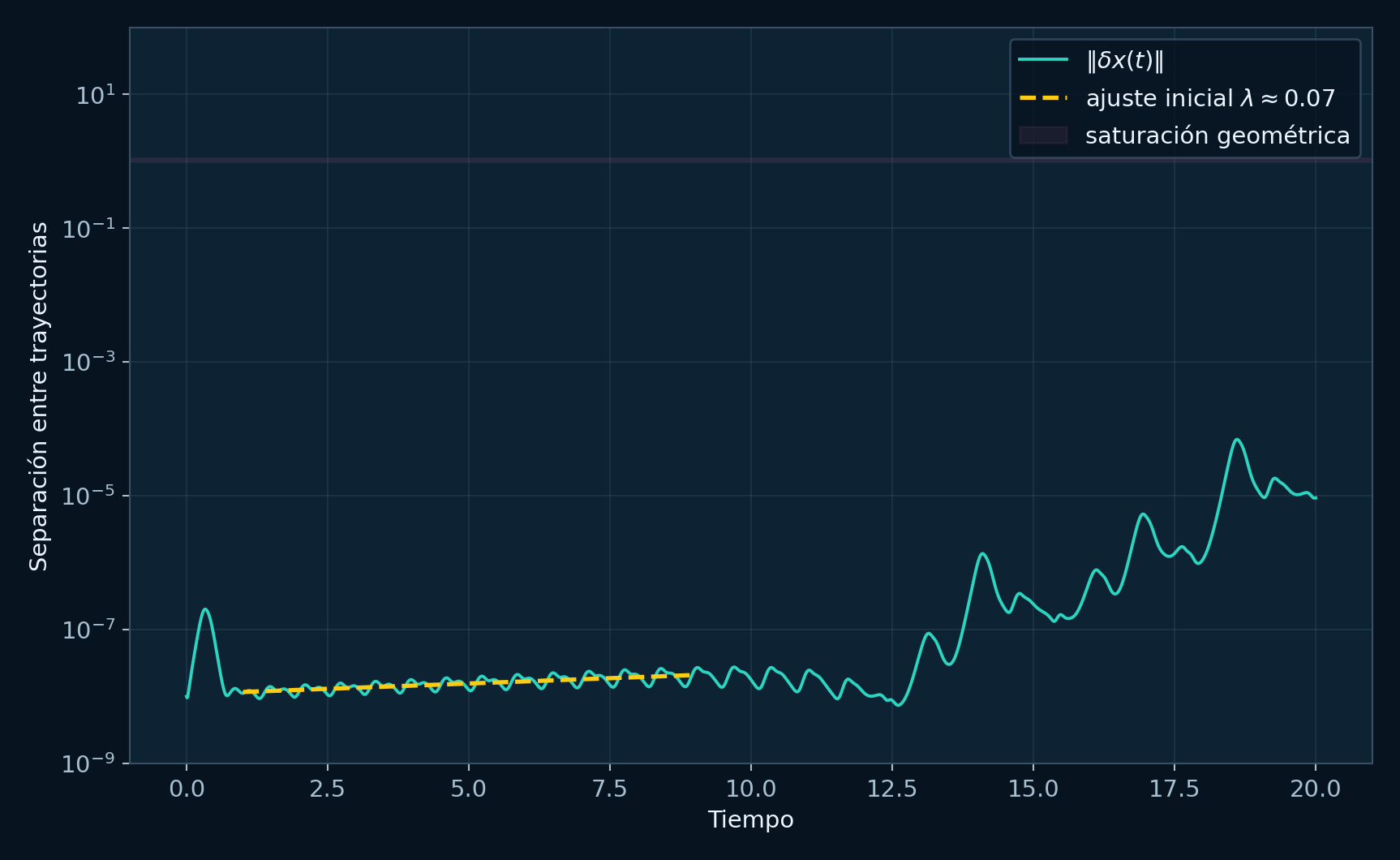
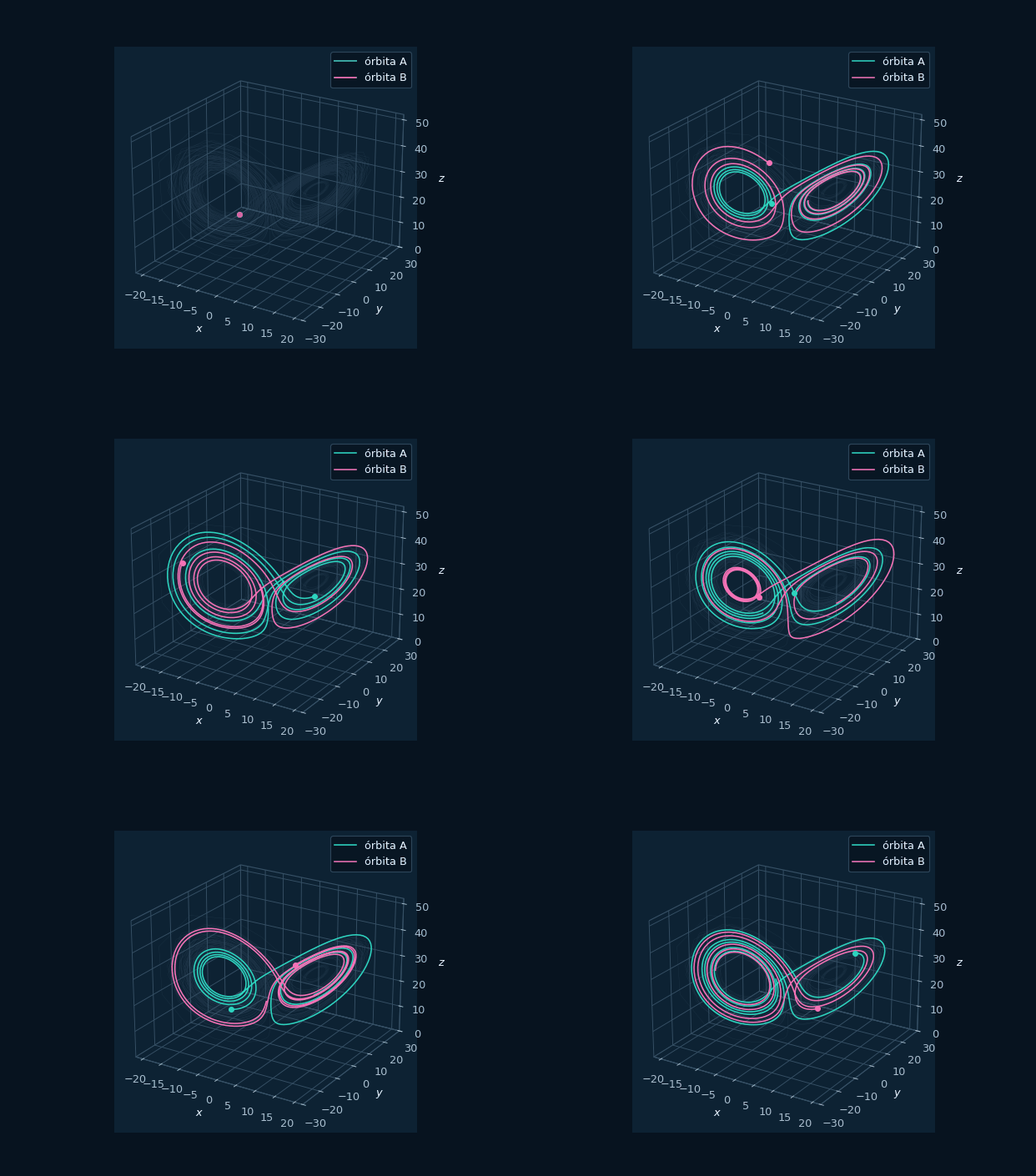
La sensibilidad describe cómo una perturbación inicial pequeña puede crecer. Para una dirección v, la ecuación variacional del flujo es $\dot v=J(x(t))v$ . El exponente máximo idealiza la tasa asintótica:

\lambda_{\max}=\lim_{t\to\infty}\frac1t\log\frac{\|\delta x(t)\|}{\|\delta x(0)\|}

En el cálculo se integran el estado y vectores tangentes, se ortogonalizan periódicamente y se acumulan logaritmos de estiramiento. Un exponente positivo sostenido respalda sensibilidad promedio; en un flujo autónomo acotado suele aparecer uno cercano a cero en la dirección temporal, y la suma negativa se relaciona con contracción de volumen.

La divergencia del campo mide la tasa infinitesimal de cambio de volumen. Para Lorenz es constante:

\nabla\!\cdot f=-\sigma-1-\beta<0

Esto muestra disipación de volumen; la sensibilidad se estudia mediante Lyapunov. Use dt=0.01, descarte 5 unidades, integre 40 y ortogonalice cada 10 pasos; repita con dt=0.005 y un horizonte mayor. Lea la curva acumulada: un número final con deriva requiere ampliar la ventana.

Separación de dos trayectorias de Lorenz con condiciones iniciales cercanas — Observe primero el intervalo en que la separación crece aproximadamente de forma exponencial y después su saturación por el tamaño finito de la región visitada. El exponente se estima en la etapa de crecimiento mediante renormalizaciones.

Ejercicio 5. Explique por qué dos trayectorias de Lorenz con inicios separados 10⁻⁶ dejan de superponerse, aunque ambas permanezcan en una región similar. Distinga error de predicción puntual y estabilidad de propiedades estadísticas.

Módulo 6 · Retornos, frecuencia y cuencas

Tres diagnósticos para tres preguntas

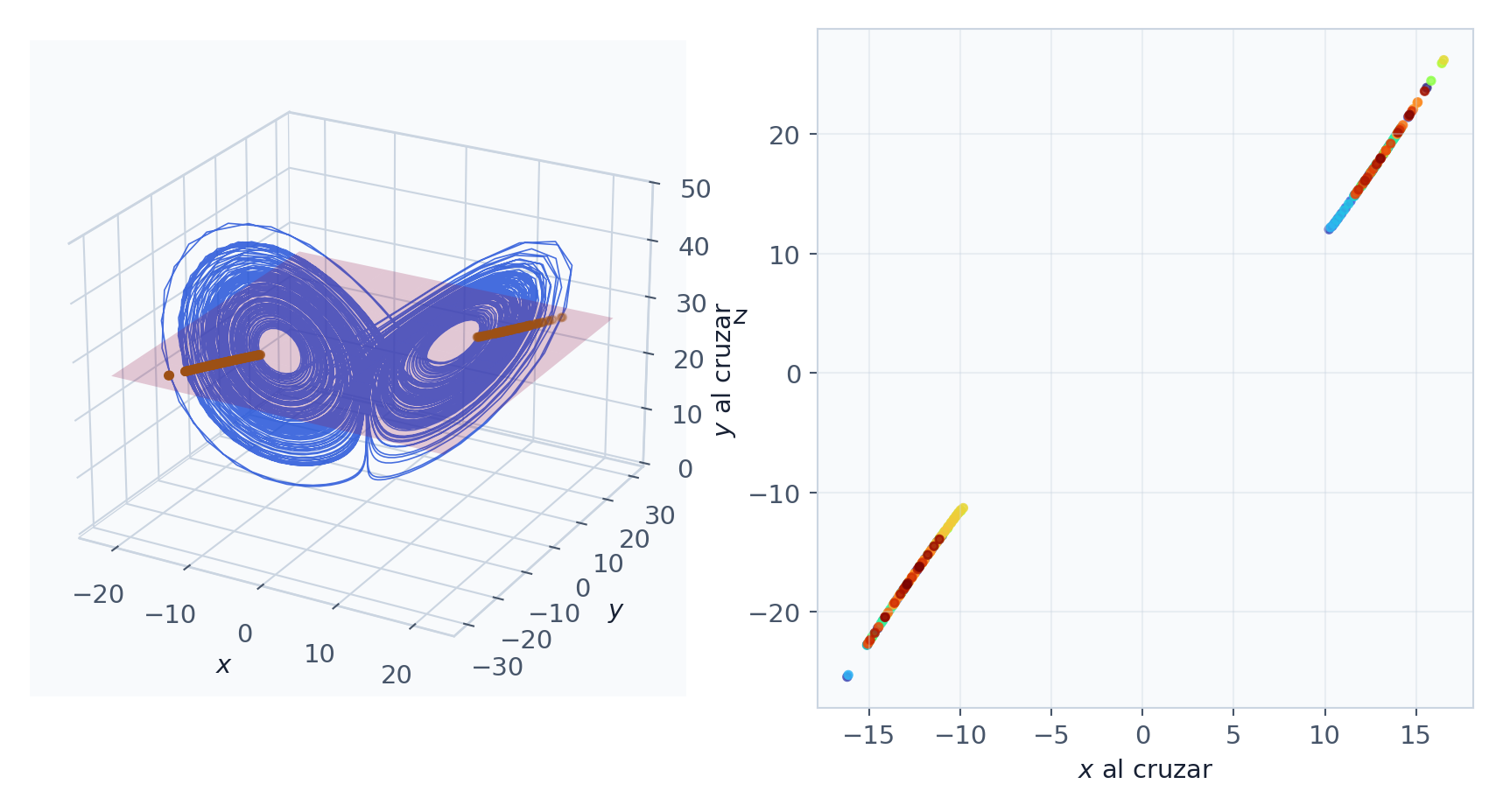
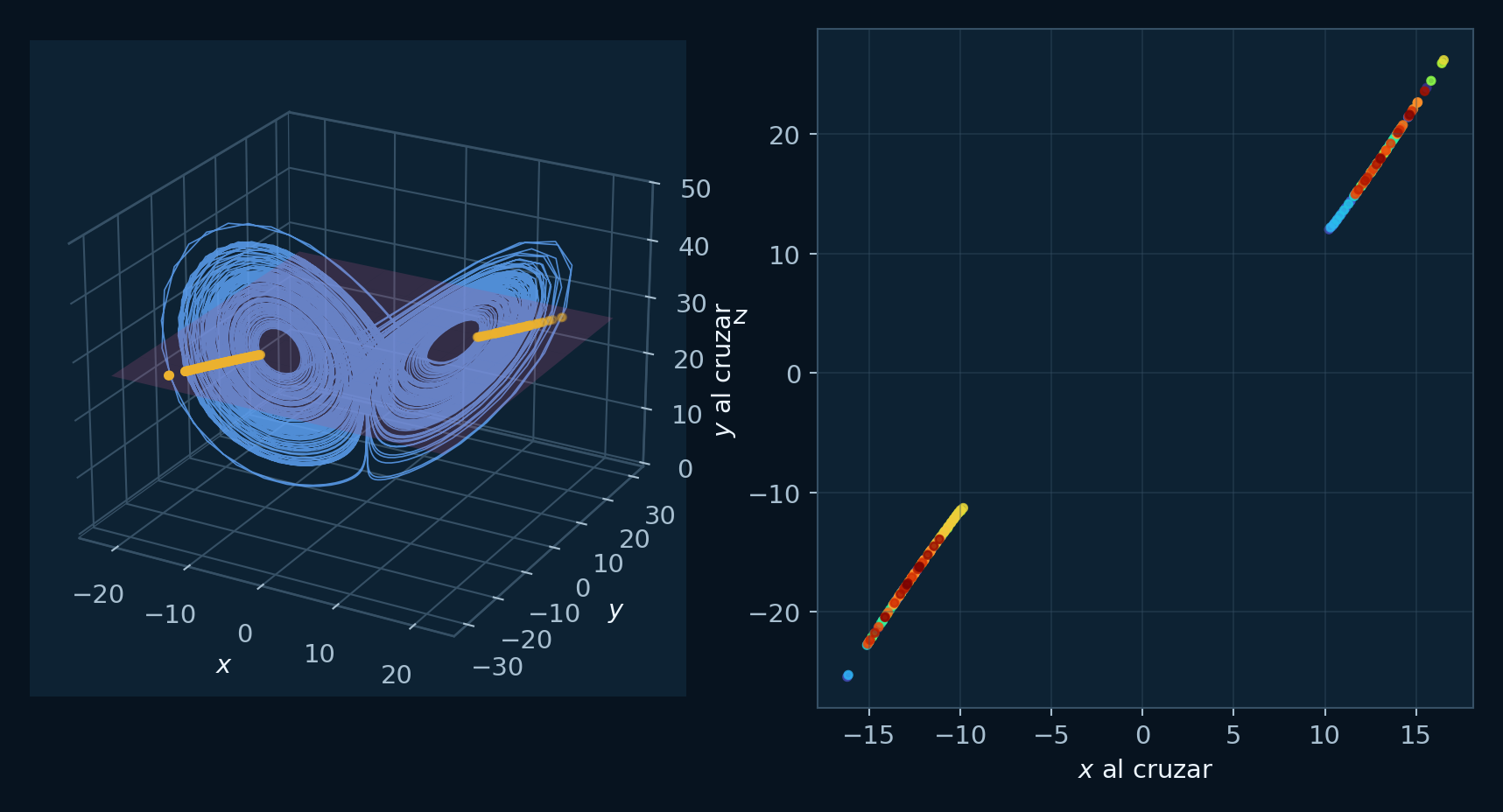
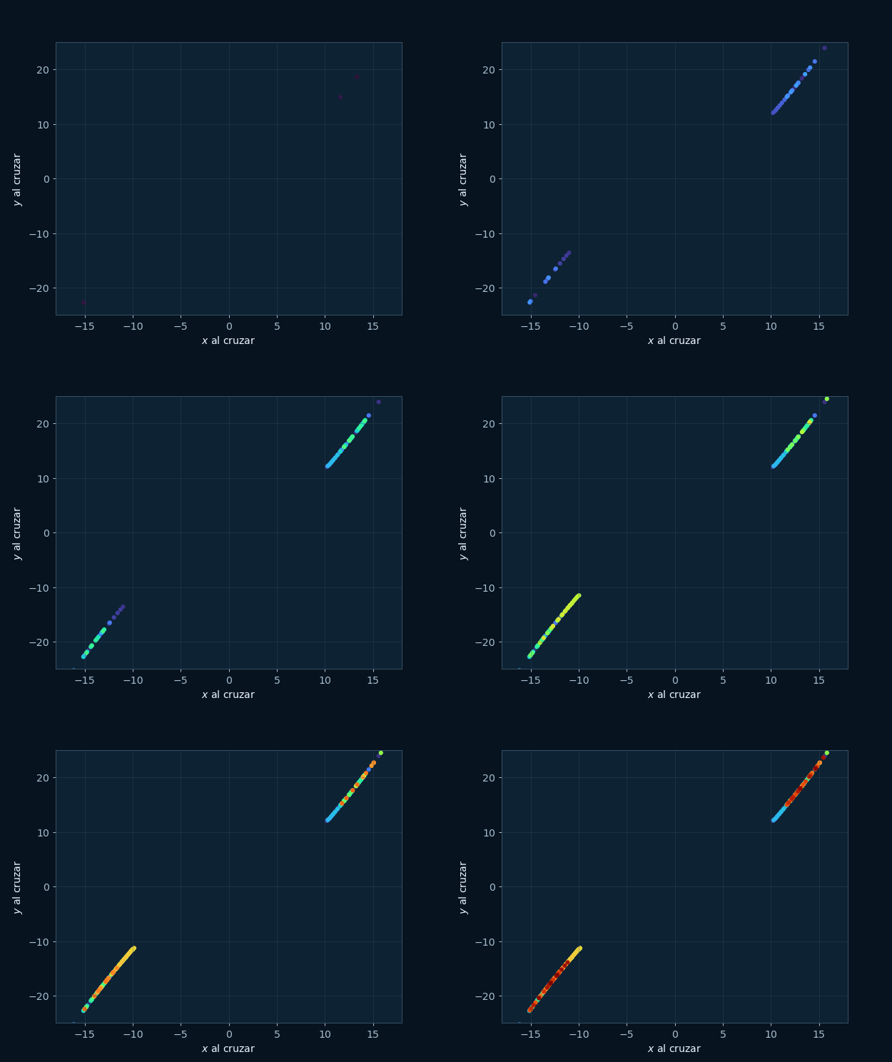
Una sección de Poincaré registra los cruces orientados de una órbita con una superficie. Convierte un flujo en un mapa de retorno y permite comparar una órbita periódica, que produce pocos puntos, con una estructura más compleja. El plano, la orientación y la interpolación del cruce forman parte de la definición; cambiarlos cambia la colección de retornos.

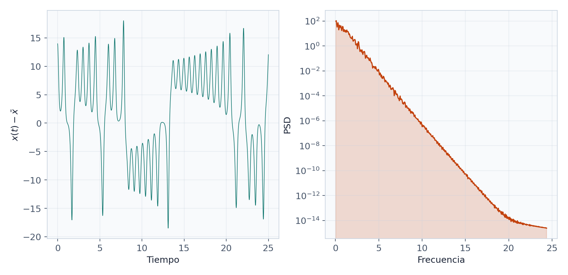
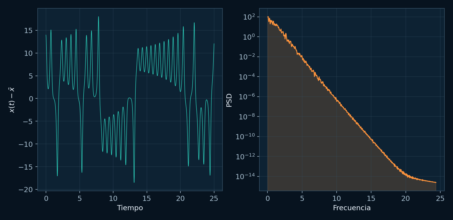
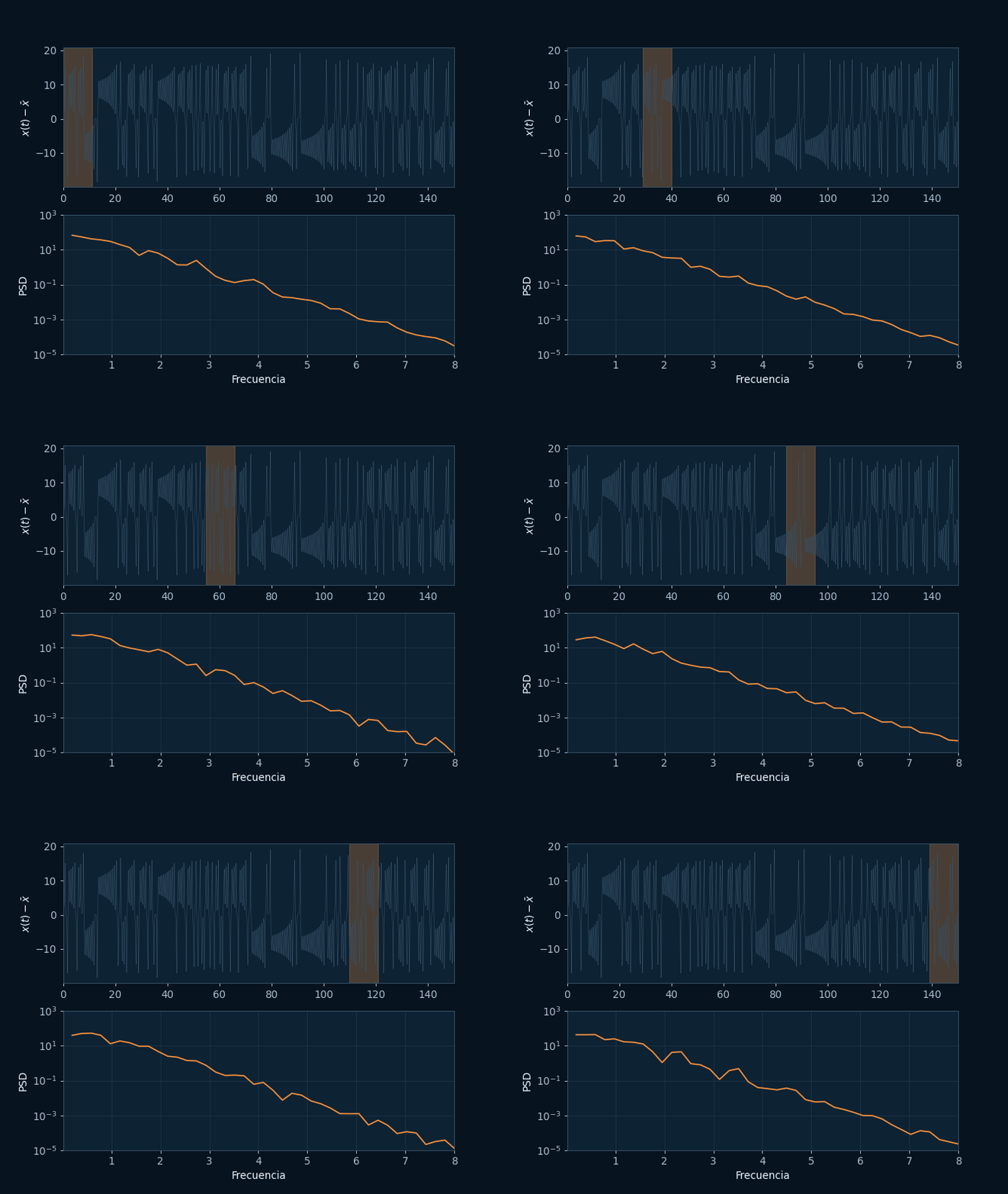
El análisis espectral responde dónde se distribuye la potencia de una serie muestreada. Para muestras xj con separación Δt, la transformada discreta usa frecuencias $f_k=k/(N\Delta t)$ . La PSD de Welch divide la señal en segmentos, aplica ventanas y promedia periodogramas, reduciendo varianza a costa de resolución. Picos estrechos son compatibles con periodicidad; potencia extendida sobre bandas es compatible con irregularidad, pero ninguna forma espectral aislada clasifica toda la dinámica.

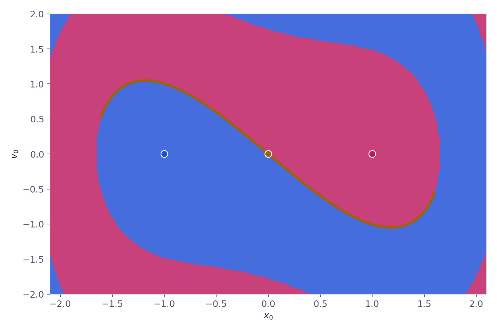
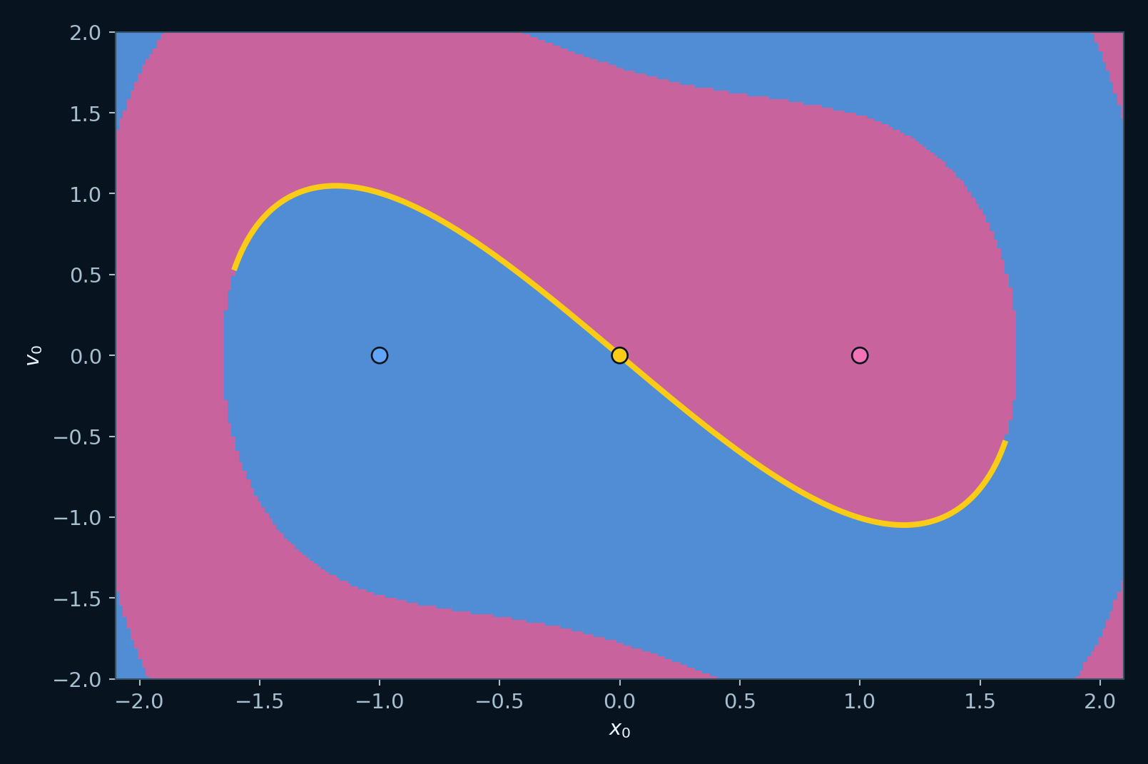
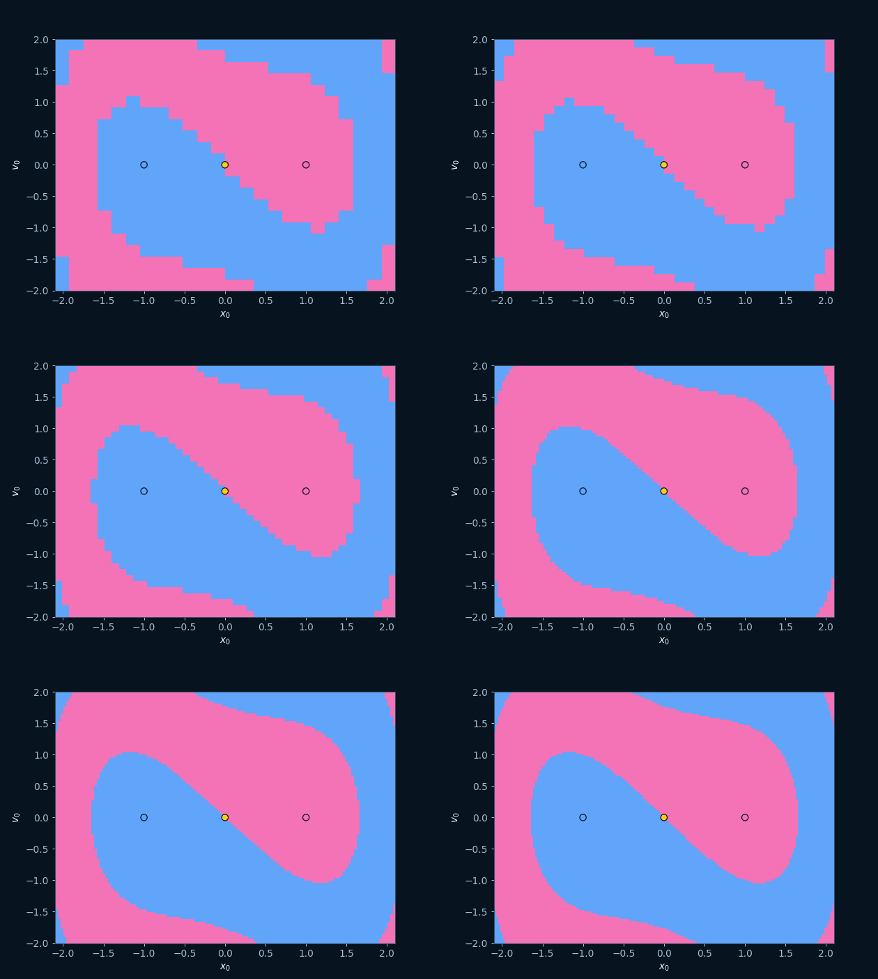
Una cuenca responde una pregunta espacial: a qué destino llega cada estado inicial de una malla bajo parámetros y horizonte fijos. Los colores codifican clases de destino; el tamaño de celda limita la frontera visible. Refinar la malla y aumentar el horizonte separa geometría persistente de píxeles debidos a resolución o convergencia lenta.

Cruces orientados de una trayectoria con una sección de Poincaré — La animación conserva sólo los cruces con la orientación elegida. Pocos puntos repetidos sugieren un retorno periódico; una nube estructurada pide estudiar el mapa de retorno y comprobar que el plano y la interpolación de cruce permanecen fijos.

Comparación visual de una serie temporal y su espectro de potencia — Al mover o ampliar la ventana cambian la resolución y la varianza espectral. Interprete picos estrechos o potencia distribuida junto con la duración, Δt, la ventana y el descarte; la geometría de la órbita se estudia con sus representaciones correspondientes.

Mapa de destinos de una cuenca biestable a distintas resoluciones — Cada color identifica el destino calculado desde un estado inicial. Active el refinamiento y distinga fronteras que persisten de detalles que sólo aparecen al reducir el tamaño de celda; el pie debe fijar plano, rango, malla, horizonte y regla de clasificación.

Ejercicio 6. Elija una serie periódica y una de Lorenz, mantenga Δt y duración, y compare PSD. Después duplique la duración. Indique qué cambios provienen de resolución frecuencial y cuáles parecen propios de la señal.

Módulo 7 · Cálculo numérico

La trayectoria calculada es una aproximación

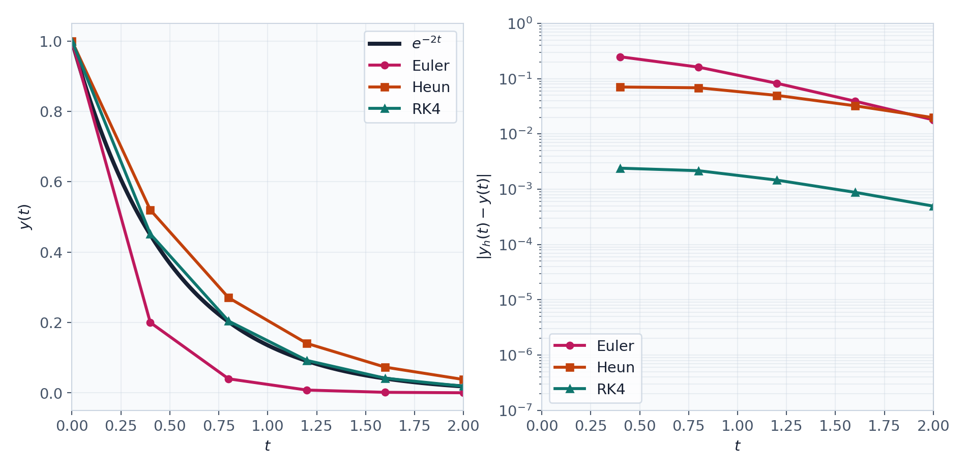
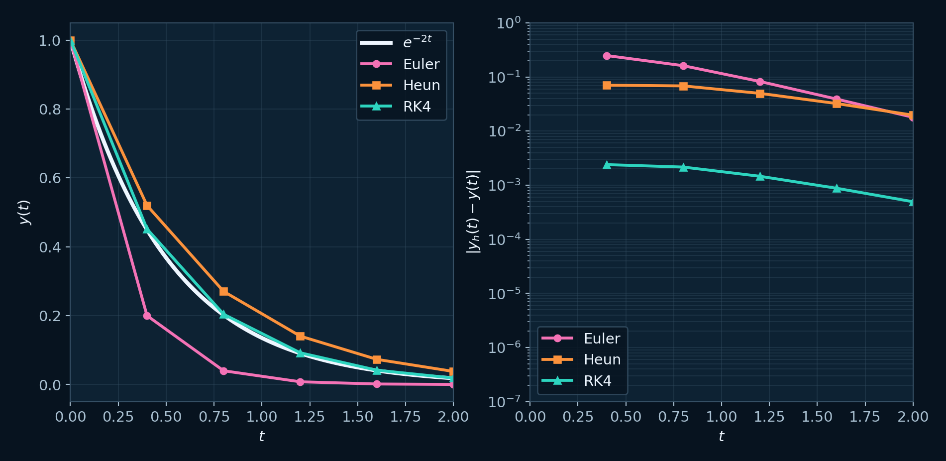
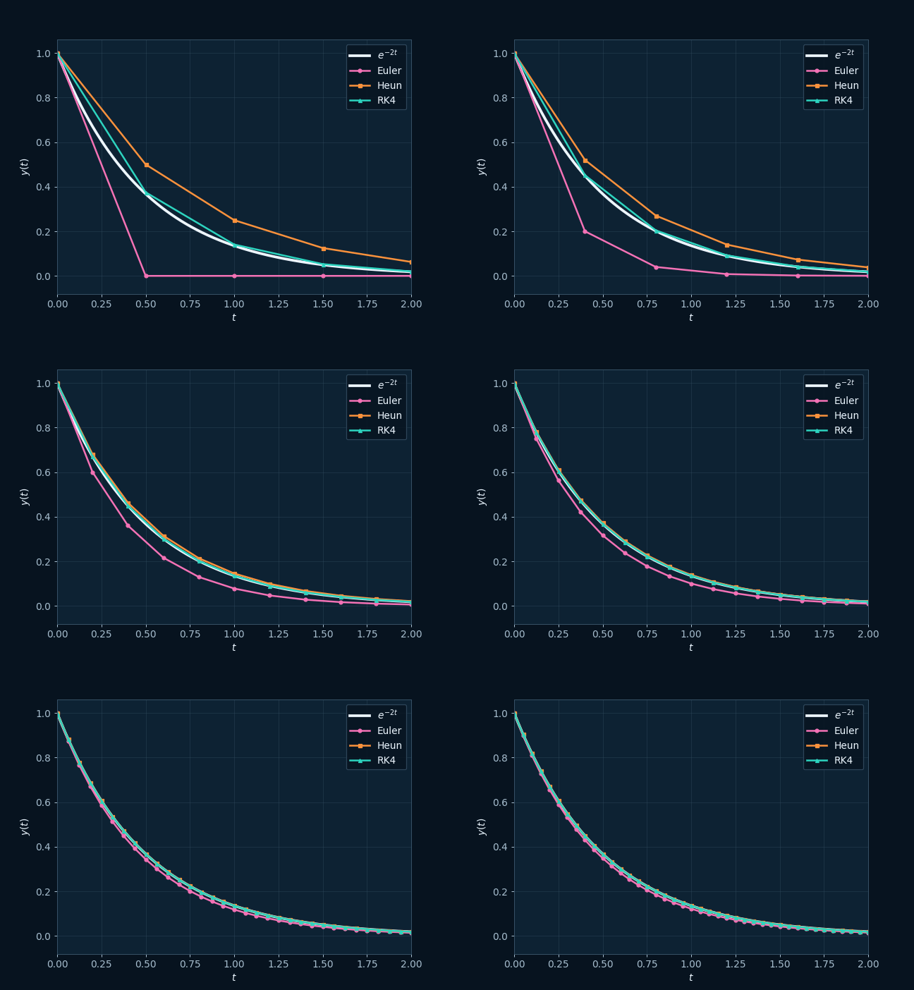
Euler aproxima la pendiente al inicio del paso, Heun promedia una predicción y una corrección, y RK4 combina cuatro pendientes. Para una EDO $\dot x=f(x)$ , sus órdenes globales son uno, dos y cuatro cuando la solución es suficientemente regular. Un método de orden alto requiere un paso compatible con la estabilidad y las escalas del sistema.

x_{n+1}^{E}=x_n+hf(x_n),\qquad x_{n+1}^{H}=x_n+\frac h2\bigl[f(x_n)+f(x_n+hf(x_n))\bigr]

La prueba de refinamiento mantiene T constante y compara h, h/2 y, si hace falta, h/4. Para una órbita sensible, la diferencia punto a punto crecerá; por ello se comparan intervalos, medias, espectros, secciones y estimaciones convergentes además del error temprano. Cuando una forma cambia al pasar de Euler a Heun o RK4, atribúyala al esquema y continúe la verificación del modelo.

Abra Comparación de métodos con Rössler a=0.2, b=0.2, c=5.7, x0=(0.1,0,0), dt=0.01 y T=80. Repita con dt=0.005. Observe primero las diferencias tempranas, luego los rangos conservados y finalmente la geometría.

Comparación de trayectorias calculadas con distintos integradores y pasos — Mire primero el intervalo temprano, donde una referencia fina permite reconocer error numérico, y luego la geometría resumida. Al reducir h debe conservarse T; las trayectorias sensibles tardías se comparan mediante las propiedades que convergen.

Ejercicio 7. A partir de una expansión de Taylor, compruebe que el error local de Euler es O(h²). Explique por qué acumular aproximadamente T/h pasos produce un error global O(h).

Módulo 8 · Lectura científica de gráficas

De la imagen a una afirmación delimitada

Una buena interpretación empieza nombrando la pregunta. La serie temporal muestra convergencia, oscilación, deriva o irregularidad en el tiempo. El retrato de fase muestra geometría y regiones visitadas. El diagrama de bifurcación compara respuestas posteriores al transitorio al variar un parámetro. La sección registra retornos. La PSD resume potencia por frecuencia. La cuenca compara destinos desde muchos inicios. Lyapunov estima tasas de expansión y contracción.

Después revise el contrato: ecuaciones, parámetros, inicio, método, paso o iteraciones, horizonte, transitorio y ajustes propios del diagnóstico. Formule una observación literal —por ejemplo, “la serie refinada permanece acotada en el intervalo mostrado”— y distingála de la interpretación —“la estimación positiva estabilizada es compatible con sensibilidad promedio”—. Cierre con las mediciones pendientes que delimitan el alcance del resultado.

El informe final del curso debe contener Lorenz, el mapa logístico y un tercer sistema elegido del catálogo. Para cada uno incluya una predicción analítica, dos gráficas complementarias, una prueba de refinamiento, una tabla de ajustes y un párrafo de límites. Use la guía de laboratorios reproducibles como recetario y continúe en el curso completo de Fyskode Learning para ejercicios y desarrollo adicional.

Comparación de proyecciones de Lorenz, Rössler y Sprott — Tres geometrías llamativas pueden requerir diagnósticos distintos. Describa primero ejes, regiones visitadas y escala; después conecte la forma con series, retornos, espectros, Lyapunov y refinamiento. La igualdad de mecanismos se establece mediante esas mediciones.

Proyecto integrador. Redacte un informe que otra persona pueda repetir a partir del protocolo escrito. Intercambie el protocolo con un compañero y complete en la bitácora cada valor y convención antes de comparar figuras.

Comprobación

Resultados breves de los ejercicios analíticos

En el ejercicio 1, los puntos fijos logísticos son 0 y 1−1/r; para r=2.8 el segundo tiene derivada 2−r=−0.8 y es estable, mientras que el origen tiene derivada r y es inestable. En el ejercicio 3, los equilibrios de x−x³ son −1, 0 y 1; f′(±1)=−2 y f′(0)=1. En el ejercicio 4, la pitchfork tiene x*=0 para todo μ y x*=±√μ cuando μ≥0; el origen cambia de estabilidad en μ=0 y las ramas no nulas son estables para μ>0. En el ejercicio 7, Taylor añade $\tfrac12h^2x''(\xi)$ al paso de Euler; repetir O(1/h) pasos explica el orden global.