Diagnósticos de Lyapunov

Calcule exponentes de Lyapunov y visualice cómo se expanden o contraen pequeñas perturbaciones en los sistemas simulados.

Nivel de dificultad Intermedio

Pregunta ¿Crecen las perturbaciones?

Pregunta y resultado

Cálculo que realizará

Estimar un espectro de Lyapunov a tiempo finito para un flujo 3D compatible bajo el contrato fijo RK4 QR–Benettin de la pestaña y decidir si los signos informados muestran suficiente convergencia numérica para sustentar un estudio posterior.

Pestaña de la interfaz

Lyapunov

Configuración y cálculo

Secuencia de controles

Seleccione un flujo compatible y reproduzca los mismos parámetros y la misma condición inicial empleados en su trayectoria.
Use el control dt propio del panel Lyapunov con un valor conservador y defina el burn-in, el tiempo final y el intervalo de renormalización QR. El cálculo sigue su contrato RK4 de paso fijo junto con los controles compartidos del sistema.
Calcule el espectro e inspeccione las curvas de convergencia en vez de leer únicamente los valores finales.
Repita con un tiempo final mayor, un burn-in ajustado y un dt menor; compare si se estabilizan los signos y los valores aproximados.

Registro

Datos obtenidos

Tres estimaciones de exponentes a tiempo finito para un flujo 3D compatible y curvas que muestran cómo evolucionan durante la acumulación.
Para el caso clásico de Lorenz, un patrón numéricamente estable con una dirección positiva, una cercana a cero y una negativa después de un refinamiento adecuado.

Lectura científica

Criterios de interpretación

Una estimación máxima positiva y estable respalda dependencia sensible para la trayectoria y el protocolo numérico probados; las direcciones cercana a cero y negativa aportan información de consistencia para un flujo continuo.

Curvas con deriva, signos cambiantes o una fuerte dependencia del paso identifican los controles que requieren refinamiento antes de formular una afirmación científica.

Archivos

Registro del experimento

Guarde la figura de convergencia junto con los valores finales de los exponentes mostrados.
Registre el sistema, los parámetros ordenados, el estado inicial, el algoritmo fijo RK4 QR–Benettin, el dt del panel Lyapunov, el burn-in, el tiempo final, el intervalo QR, la versión del software y cada ejecución de refinamiento utilizada en la interpretación.

Aplicaciones

Preguntas que admite el cálculo

Respaldar análisis de sensibilidad después de inspeccionar la trayectoria y los transitorios.
Comparar la convergencia numérica entre parámetros, horizontes temporales y pasos de integración.
Enseñar expansión local, dirección neutra del flujo, contracción e incertidumbre a tiempo finito.

Alcance

Condiciones de la evidencia

Los exponentes a tiempo finito dependen de la trayectoria, la duración, la eliminación de transitorios, el integrador y los ajustes de renormalización.
Una estimación positiva en una ejecución corta requiere controles de transitorio, paso y convergencia antes de sostener una interpretación de caos.
Esta pestaña estima separación a tiempo finito; complete atracción, estructura de cuencas, unicidad y localización de atractores ocultos con los procedimientos específicos, incluidos los de Hidden Attractors FO cuando corresponda.

Separación a escala logarítmica de dos trayectorias cercanas del sistema de Lorenz — Animación con la trayectoria libre de título incrustado: dos trayectorias de Lorenz casi idénticas se separan primero de manera aproximadamente exponencial. La pendiente del tramo inicial aporta una tasa a tiempo finito; la saturación posterior indica que la distancia alcanzó la escala del atractor.

Separación entre dos trayectorias de Lorenz y ajuste del crecimiento inicial — Lectura cuantitativa: en el eje vertical logarítmico, un tramo aproximadamente recto permite estimar una pendiente local. El ajuste se hace antes de la saturación geométrica y debe repetirse al refinar paso, transitorio y horizonte.

Pestaña Lyapunov de Toolbox Chaos mostrando el espectro de Lorenz a tiempo finito — Interfaz actual: el espectro de Lorenz a tiempo finito se muestra junto con todas las curvas de convergencia y el contrato de integración.

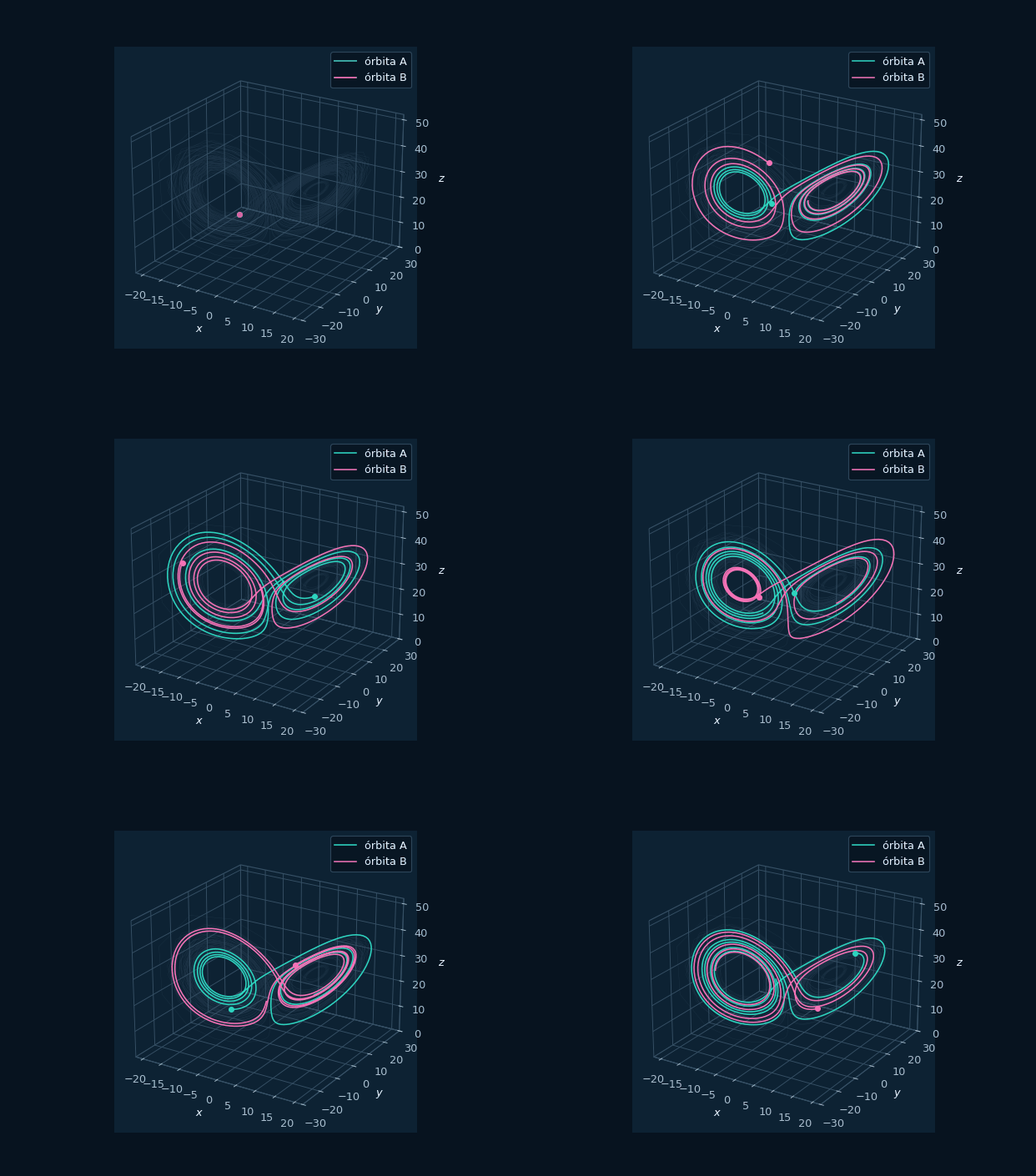
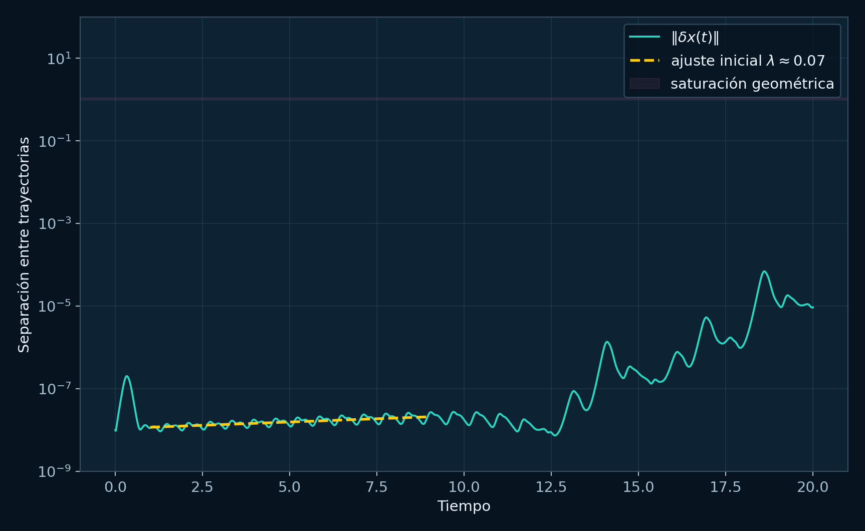
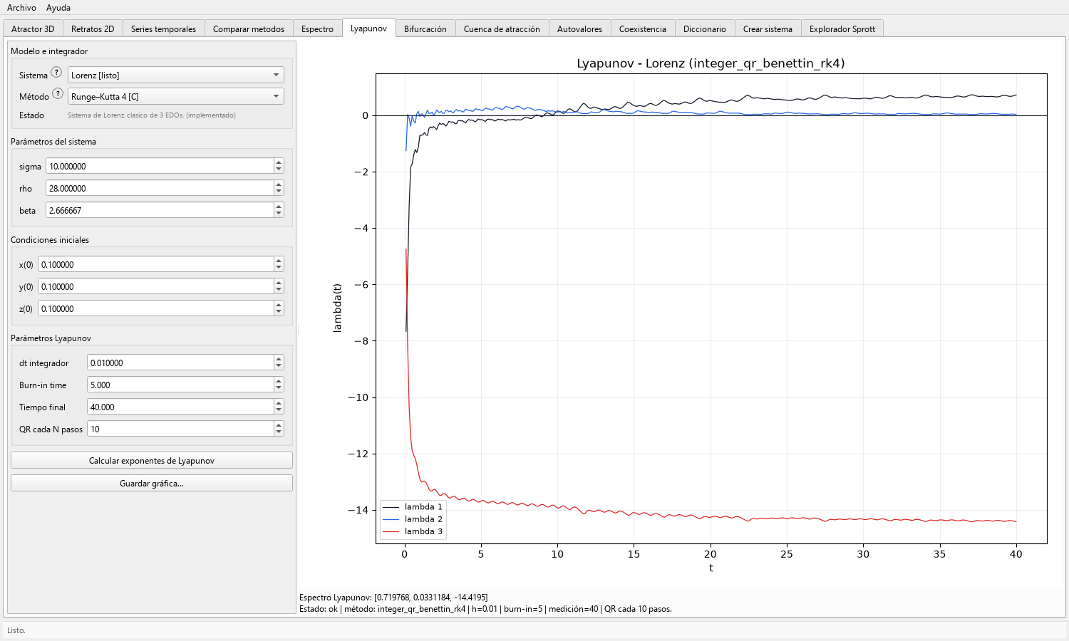
Configuración QR--Benettin y convergencia

Abra el flujo de trabajo Lyapunov en Toolbox Chaos.
Seleccione el flujo objetivo y conserve los mismos parámetros utilizados para la gráfica de la trayectoria.
El cálculo de Lyapunov usa un algoritmo RK4 QR–Benettin de paso fijo. Defina su dt específico de forma conservadora; para Lorenz, dt = 0.01 es un primer valor práctico. Este cálculo sigue su contrato RK4 dedicado.
Use un intervalo de burn-in antes de acumular las estimaciones de los exponentes.
Ejecute una ventana de integración suficientemente larga antes de interpretar el exponente máximo.
Inspeccione la gráfica de convergencia junto con el número final.
Informe el espectro como evidencia numérica y acompañe una ejecución corta con los controles de convergencia correspondientes.

Exponentes de Lyapunov a tiempo finito

Los exponentes de Lyapunov miden tasas exponenciales promedio de separación o contracción entre estados cercanos en el espacio de fases. El número de exponentes coincide con la dimensión del sistema. Un exponente máximo positivo es evidencia numérica de dependencia sensible respecto de las condiciones iniciales.

Para un flujo continuo tridimensional, un espectro caótico típico tiene un exponente positivo, uno cercano a cero y uno negativo. La dirección cercana a cero corresponde al movimiento a lo largo de la propia trayectoria; la dirección negativa registra contracción.

Las curvas de convergencia son importantes porque las estimaciones a tiempo finito pueden derivar. Se debe comprobar si las estimaciones se estabilizan al refinar el burn-in, el tiempo final y el paso de integración.

El contrato numérico de esta pestaña es QR–Benettin de orden entero con un integrador RK4 fijo. Informe el dt específico de Lyapunov, el burn-in, el tiempo de medición y el intervalo QR mostrados con el resultado, e identifique el cálculo como QR–Benettin con RK4 fijo.

Parámetros de la estimación de Lyapunov

Burn-in: un burn-in insuficiente permite que el comportamiento inicial sesgue la estimación de los exponentes.
Tiempo total: las integraciones cortas pueden producir un signo incorrecto o valores inestables.
Tamaño de paso: un paso grande puede crear expansión o contracción artificial.
Tamaño de la perturbación: las perturbaciones deben permanecer suficientemente pequeñas para aproximar el comportamiento tangente local.
Intervalo de renormalización: si los vectores se renormalizan con muy poca frecuencia, pueden desbordarse o colapsar en una dirección.
Condición inicial: los transitorios de larga duración o la multiestabilidad pueden cambiar el espectro observado a tiempo finito.