Diagramas de bifurcación

Configura barridos de parámetros, puntos conservados, secciones de Poincaré y ejemplos de Hopf para visualizar cambios cualitativos en la dinámica.

Nivel de dificultad Principiante

Pregunta ¿Qué cambia al modificar un parámetro?

Pregunta y resultado

Cálculo que realizará

Barrer un parámetro del modelo, conservar un observable controlado de largo plazo e identificar intervalos que merecen una simulación más detallada.

Pestaña de la interfaz

Bifurcación

Configuración y cálculo

Secuencia de controles

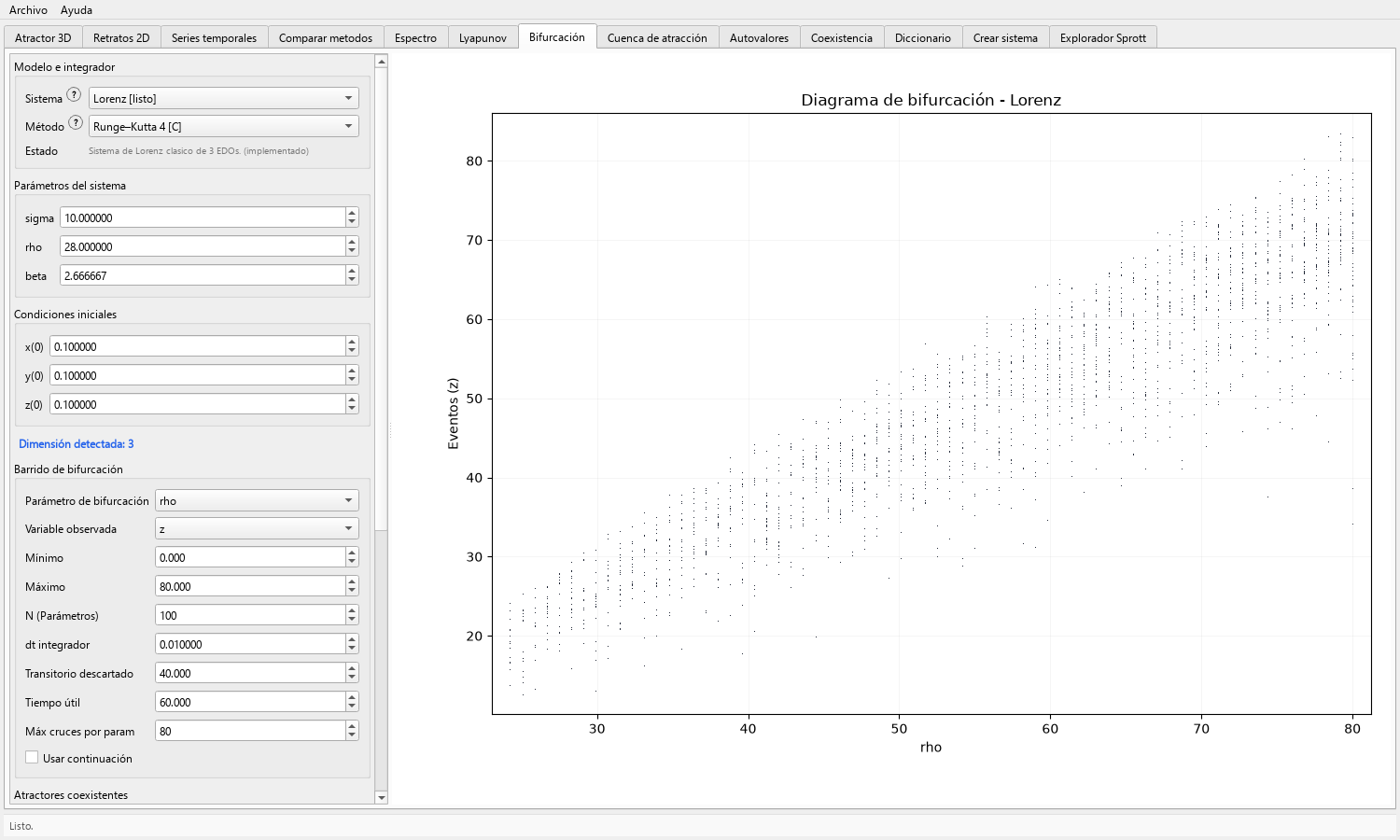
Selecciona el sistema, el parámetro que se barrerá y la variable observada; después define el mínimo, el máximo y el número de muestras del parámetro.
Establece el paso de integración, el transitorio descartado, el tiempo útil y el máximo de cruces o valores conservados por parámetro.
Activa Usar continuación cuando cada valor del parámetro deba iniciar desde el estado final obtenido en el valor anterior; déjala desactivada para reiniciar desde la condición inicial declarada en cada valor.
Activa Comparar atractores coexistentes para ejecutar el mismo barrido desde las condiciones iniciales A y B; selecciona ambos casos registrados o edita sus coordenadas y asigna colores contrastantes.
Calcula el diagrama, repite con un intervalo local más denso cuando sea necesario y compara la continuación activada y desactivada cuando la dependencia de la trayectoria pueda afectar las ramas.
Exporta solo después de registrar el intervalo del parámetro, la densidad de muestreo y el observable graficado.

Registro

Datos obtenidos

Una nube de puntos parámetro-observable que muestre ramas, cruces o bandas densas de respuesta conservadas.
Con la continuación activada, un barrido que siga el estado alcanzado numéricamente de un valor del parámetro al siguiente.
En el modo A/B, dos conjuntos de datos etiquetados y superpuestos con los mismos controles de barrido para comparar su dependencia de las condiciones iniciales.

Lectura científica

Criterios de interpretación

La división de ramas y las bandas densas permiten identificar cambios cualitativos que conviene examinar, pero su apariencia depende del observable, el transitorio, la regla de muestreo, la dirección del barrido y la configuración numérica.

Una diferencia entre la continuación y los reinicios independientes es evidencia de dependencia respecto de la trayectoria o del estado inicial en el barrido finito. Una clasificación global requiere un análisis con cobertura declarada.

La separación entre los conjuntos A y B documenta los dos inicios declarados y la trayectoria de parámetros ensayada. Amplíe la muestra para estudiar otras respuestas coexistentes.

Archivos

Registro del experimento

Usa Guardar gráfica... después de comprobar que las etiquetas de los ejes y las regiones densas sean legibles al tamaño previsto de publicación.
Registra el sistema, los parámetros ordenados, el parámetro barrido y su intervalo, la variable observada, N, el método, dt, el transitorio, el tiempo útil, el máximo de puntos, el estado de continuación y, cuando corresponda, las condiciones iniciales, etiquetas y colores A/B.

Aplicaciones

Preguntas que admite el cálculo

Localizar ventanas de parámetros para estudiar después trayectorias, espectros o diagnósticos de Lyapunov.
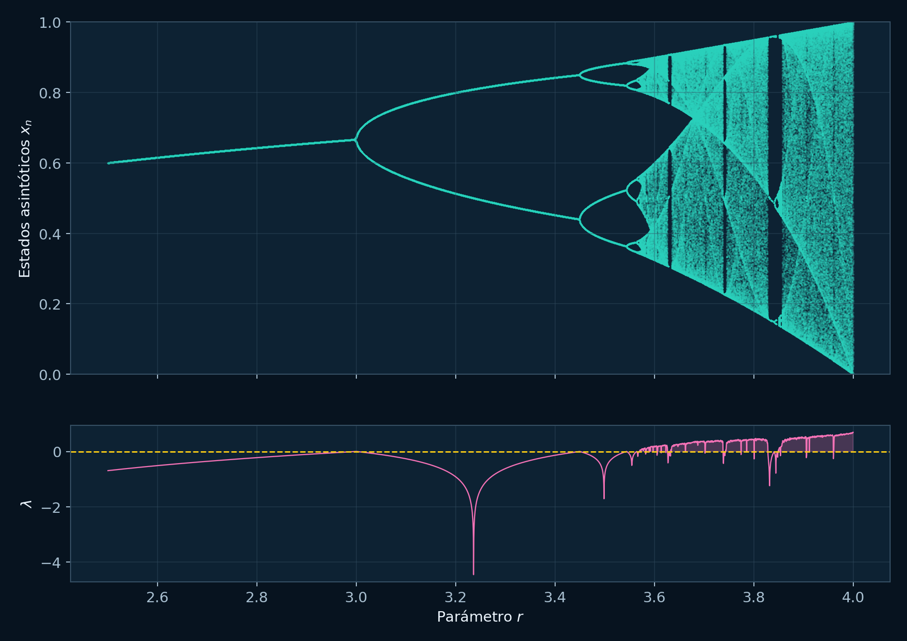
Enseñar ramas fijas, cambios de periodo, estructuras de retorno y el efecto del diseño del barrido.
Comparar métodos numéricos o intervalos experimentales de parámetros con una regla de medición común.

Alcance

Condiciones de la evidencia

Una rama con apariencia de bifurcación puede alterarse por un descarte insuficiente del transitorio, un muestreo grueso, un paso de integración grande o el observable elegido.
La continuación puede seguir una rama alcanzable y omitir alternativas; un reinicio independiente también puede omitir estados fuera de la condición inicial elegida.
La comparación A/B muestrea dos inicios declarados. Una búsqueda ampliada declara la colección de inicios y respuestas analizadas.
El diagrama organiza respuestas frente a un parámetro; establezca caos, atracción, unicidad o carácter oculto mediante los análisis específicos de cada propiedad.

Pestaña Bifurcación actual de Toolbox Chaos con un barrido de rho en Lorenz — Interfaz actual: un barrido de rho de densidad moderada para Lorenz conserva eventos de Poincaré después del transitorio declarado.

Diagrama de bifurcación del mapa logístico y multiplicador del punto fijo — Referencia de lectura: el panel superior reúne estados asintóticos después del transitorio; el inferior sigue el multiplicador local. Las ramas separadas indican periodicidad y las bandas densas exigen pruebas adicionales antes de llamarlas caos.

Trayectoria de Lorenz y puntos de retorno sobre una sección de Poincaré — Sección de Poincaré: una trayectoria continua de Lorenz se reduce a puntos de retorno sobre un plano seleccionado. Esta representación compacta permite comparar la estructura recurrente declarada.

Amplitud del ciclo y retratos de fase de una bifurcación de Hopf supercrítica — Ejemplo de Hopf: la amplitud es cero antes del umbral y crece como una raíz cuadrada después de él; los retratos de fase muestran la transición local del equilibrio al ciclo. Una ruta al caos requiere su propio barrido y diagnósticos.

Barrido paramétrico y registro de respuestas

Abre el flujo de trabajo de bifurcación en Toolbox Chaos.
Selecciona el sistema que se barrerá. Comienza con Logistic para un ejemplo rápido de mapa o con Lorenz para un ejemplo de flujo.
Elige el parámetro de control, por ejemplo r para Logistic o rho para Lorenz.
Define primero un intervalo grueso, como r = 2.8 a 4.0 para Logistic o rho = 0 a 60 para Lorenz.
Descarte suficiente comportamiento transitorio para que la gráfica muestre valores conservados de largo plazo y registre el intervalo inicial apartado.
Elige cómo se inicializa el barrido: con Usar continuación activado, el estado final de un valor del parámetro se convierte en el inicio del siguiente; desactivado, cada valor reinicia desde la condición inicial declarada. Compara ambas configuraciones cuando la selección de ramas sea relevante.
Para una comparación controlada de dos inicios, activa Comparar atractores coexistentes, elige Atractor A y Atractor B, verifica ambas ternas de condiciones iniciales y selecciona colores contrastantes. La pestaña aplica el mismo barrido y la misma configuración numérica a ambos conjuntos.
Aumenta el número de muestras del parámetro y de puntos conservados solo cuando el intervalo ya sea significativo.
Exporta una figura grande cuando las ramas y las regiones densas sean legibles.

Respuestas retenidas y transiciones locales

Un diagrama de bifurcación resume visualmente cómo cambia un sistema dinámico cuando varía un parámetro. Para cada valor del parámetro, la simulación descarta el transitorio y grafica valores conservados de largo plazo. Una sola rama sugiere un comportamiento fijo estable; dos, cuatro o muchas ramas sugieren estructura periódica; las bandas densas sugieren regímenes irregulares o caóticos.

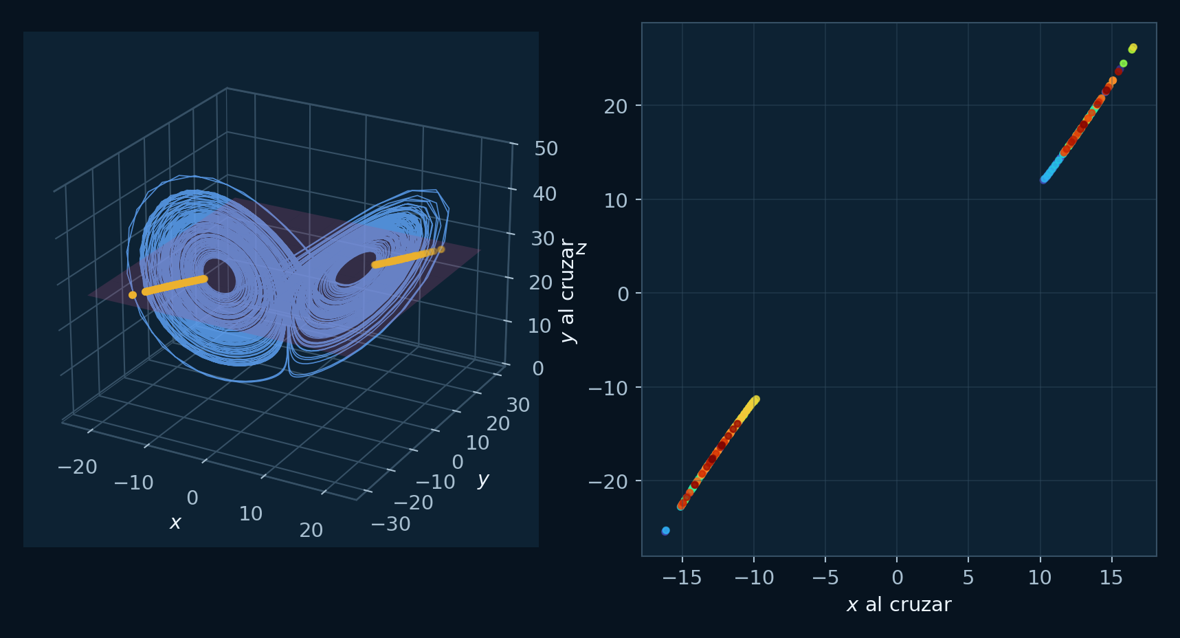
En los mapas, los valores conservados son iteraciones directas. En los flujos, Toolbox Chaos necesita una regla de evento o medición, como máximos locales, estados finales conservados o un cruce de Poincaré. Esa regla es importante porque determina qué parte de la trayectoria continua se convierte en un punto de la gráfica.

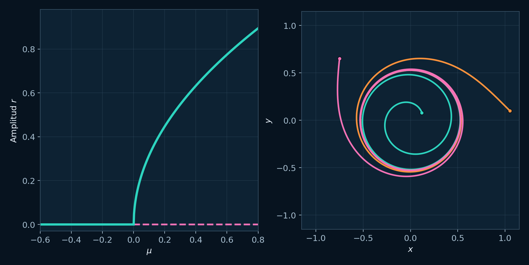
Una bifurcación de Hopf es un mecanismo local específico en el que un equilibrio cambia de estabilidad y nace o desaparece una oscilación. Pertenece a la misma familia visual de diagramas de cambio de parámetros; una ruta completa hacia el caos requiere una secuencia de evidencia propia.

Parámetros que organizan el barrido

Intervalo del parámetro: uno demasiado amplio puede comprimir ramas importantes; uno demasiado estrecho puede ocultar la ruta hacia el comportamiento que deseas mostrar.
Muestras del parámetro: muy pocas muestras hacen que el diagrama parezca vacío o irregular. Aumenta la densidad para las gráficas finales.
Duración del transitorio: si es muy corta, deja puntos iniciales en la gráfica. Aumenta el descarte antes de interpretar las ramas.
Puntos conservados: muy pocos valores ocultan bandas densas; demasiados pueden superponerse hasta formar un bloque sólido.
Paso de integración: en flujos, un paso grande puede crear artefactos numéricos que parezcan bifurcaciones.
Plano de Poincaré: cambiar el plano de sección o la dirección de cruce modifica los retornos que se grafican.