Cuencas de atracción

Calcula e interpreta mapas de cuencas sobre una malla que clasifican las condiciones iniciales según su destino final.

Pregunta ¿A dónde llega cada inicio?

Úsalo cuando Necesites una clasificación sobre una malla

Pregunta y resultado

Cálculo que realizará

Construir un mapa bidimensional de condiciones iniciales, comparar las clases de destino calculadas y verificar la interpretación mediante trayectorias representativas.

Pestaña de la interfaz

Cuenca de atracción

Configuración y cálculo

Secuencia de controles

Selecciona un flujo 3D compatible y define sus parámetros, el método de integración, el paso y el tiempo total.
Establece los límites de x0 y y0, la coordenada fija z0 y una malla Nx por Ny moderada para el primer cálculo.
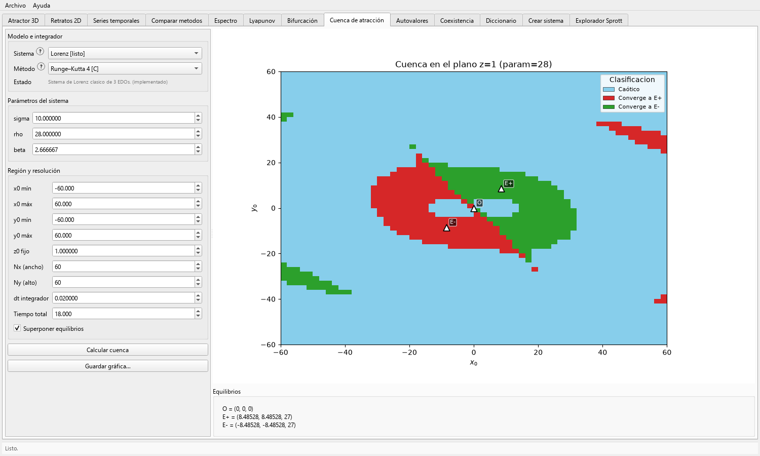
Mantén Superponer equilibrios activado cuando los marcadores de equilibrio ayuden a orientar el mapa; el panel Equilibrios muestra las coordenadas utilizadas por la vista.
Calcule la cuenca, examine las regiones de escape o pendientes de clasificación y refine la ventana, el tiempo o la resolución cuando el primer mapa delimite los controles necesarios.
Simula inicios representativos de colores distintos antes de asignar un significado dinámico a cada clase.

Registro

Datos obtenidos

Una malla codificada por colores en la que cada condición inicial muestreada recibe una clase de destino calculada.
Cuando se solicite, marcadores de equilibrio sobre el mapa y coordenadas de equilibrio seleccionables en el panel informativo adyacente.

Lectura científica

Criterios de interpretación

Los colores son etiquetas numéricas de clase para el plano, la malla, la configuración del solucionador y el tiempo finito de integración seleccionados. Los valores de las variables de estado se consultan en las trayectorias correspondientes.

La superposición de equilibrios proporciona puntos de referencia geométricos. Complétela con trayectorias representativas y pruebas de convergencia cerca de una frontera.

Archivos

Registro del experimento

Usa Guardar gráfica... para guardar la figura de la cuenca después de comprobar que su leyenda, sus límites y sus marcadores de equilibrio sean legibles.
Registra el sistema, los parámetros ordenados, el método, dt, el tiempo total, la ventana x0/y0, el valor fijo z0, Nx, Ny y si se mostraron los equilibrios superpuestos.

Aplicaciones

Preguntas que admite el cálculo

Estudiar la sensibilidad a las condiciones iniciales y las regiones de destino multiestables.
Seleccionar inicios representativos para comparar trayectorias posteriormente y enseñar el concepto de cuenca.
Comparar cómo cambia una cuenca muestreada ante variaciones controladas de parámetros o resolución.

Alcance

Condiciones de la evidencia

Una malla finita puede omitir regiones pequeñas o complejas, y un horizonte finito puede clasificar incorrectamente transitorios lentos.
La sección mostrada documenta un plano del espacio de estados; evalúe la atracción desde una vecindad con trayectorias y criterios de convergencia.
Este flujo de trabajo de la interfaz documenta cuencas muestreadas; la localización y certificación de atractores ocultos corresponde a Hidden Attractors FO.

Pestaña Cuenca de atracción actual de Toolbox Chaos con una clasificación de Lorenz — Interfaz actual: cada celda es una condición inicial sobre el plano declarado y su color indica la clase de destino a tiempo finito.

Mapa de cuencas biestable con dos clases de destino y condiciones iniciales representativas — Lectura del mapa: cada color codifica un destino observado bajo el contrato numérico declarado. Seleccione puntos a ambos lados de la frontera, reintegre y compruebe que la clasificación se conserva al refinar malla, paso y horizonte.

Estructura de una cuenca de atracción

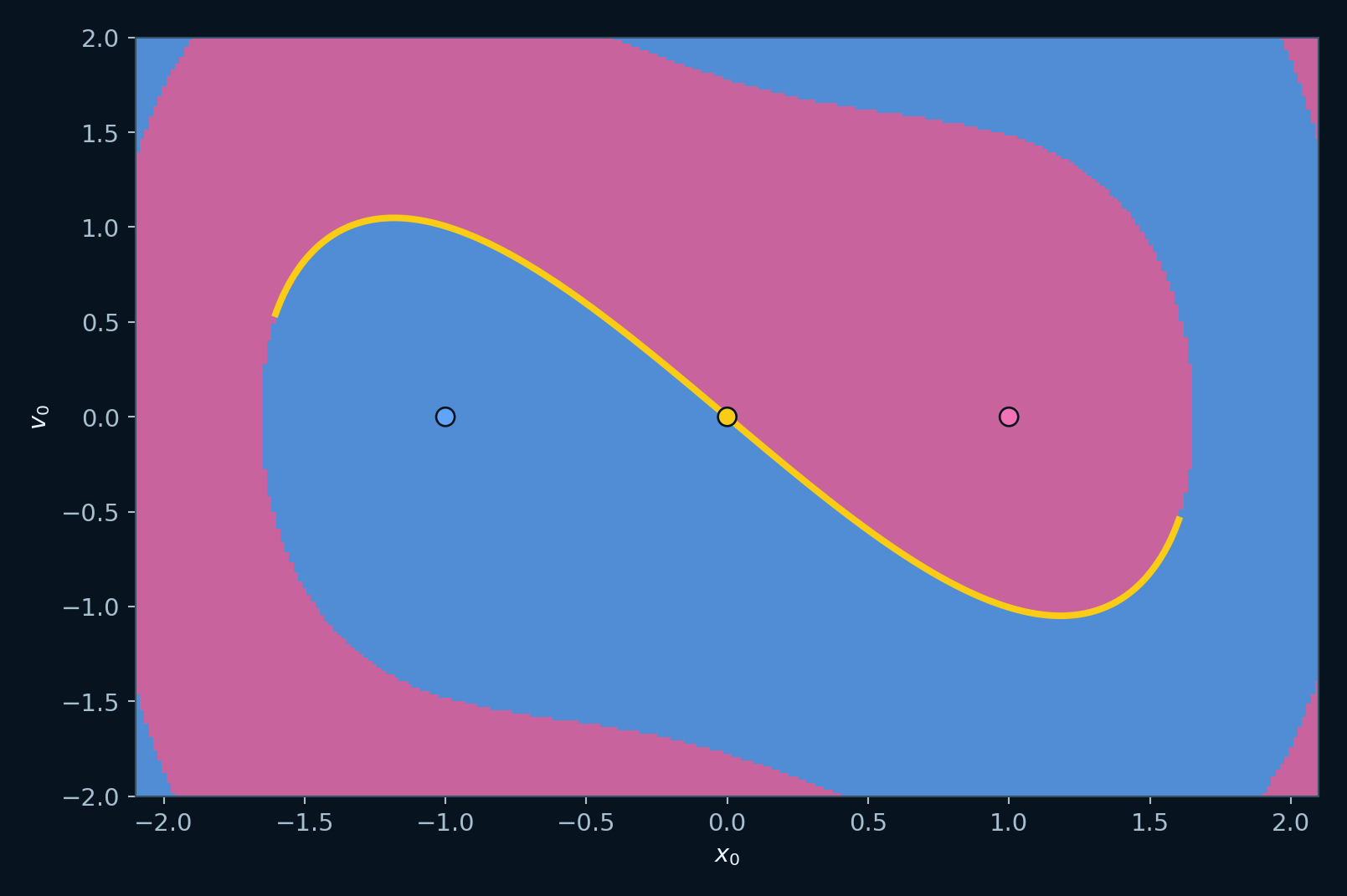
Una cuenca de atracción divide las condiciones iniciales según su comportamiento final. En una gráfica bidimensional de cuencas, los ejes horizontal y vertical representan dos coordenadas iniciales y la tercera se mantiene fija. El solucionador inicia una trayectoria desde cada punto de la malla, la integra y clasifica su destino después de la ventana de integración conservada.

Una práctica importante consiste en distinguir el mapa de las trayectorias. El mapa indica el destino de muchos inicios. Las trayectorias representativas muestran por qué los colores son significativos: los inicios elegidos en regiones distintas llegan a zonas finales diferentes.

Muestreo de condiciones iniciales y clasificación de destinos

Abre el flujo de trabajo de cuencas de atracción en Toolbox Chaos.
Selecciona un flujo continuo 3D compatible, como Lorenz, Chua o Rossler.
Elige los límites del plano con x0 min, x0 max, y0 min y y0 max.
Establece la coordenada fija, por ejemplo z0 = 1 para un plano x-y de condiciones iniciales de Lorenz.
Usa Superponer equilibrios cuando quieras mostrar marcadores de equilibrio sobre el mapa y consulta sus coordenadas en el panel Equilibrios. Desactiva la opción cuando los marcadores oculten una frontera densa.
Comienza con una malla moderada, como Nx = 120 y Ny = 120. Aumenta la resolución solo cuando la región ya sea significativa.
Ejecute la clasificación, examine las clases estables y registre los casos divergentes o pendientes de clasificación.
Elige condiciones iniciales representativas de regiones de colores distintos y simula sus trayectorias para confirmar la interpretación de la cuenca.

Parámetros que determinan el mapa

Resolución de la malla: valores mayores de Nx y Ny revelan fronteras más finas, pero aumentan el tiempo de cálculo.
Tiempo de integración: uno demasiado corto puede clasificar mal una convergencia lenta; uno demasiado largo puede encarecer las mallas de alta resolución.
Coordenada fija: al cambiarla se modifica el plano muestreado, por lo que también puede cambiar la forma de la cuenca.
Ventana del plano: una región amplia aporta contexto; una región estrecha resulta más útil después de localizar la frontera.
Umbrales del clasificador: los radios de llegada y escape, junto con las etiquetas pendientes de clasificación, controlan cómo se asignan los destinos finales.

Cuencas, coexistencia y trayectorias

Mapa de cuencas: clasifica muchas condiciones iniciales sobre una malla.
Gráfica de coexistencia: compara un conjunto pequeño de trayectorias seleccionadas con parámetros fijos.
Gráfica del atractor: muestra en el espacio de fases la geometría de largo plazo de una trayectoria.