Primeros pasos con el atractor de Lorenz

Configura los parámetros, ejecuta tu primera simulación y compara el espacio de fases 3D con retratos de fase 2D proyectados para el sistema de Lorenz.

Nivel de dificultad Principiante

Pregunta ¿Qué aspecto tiene una trayectoria?

Pregunta y resultado

Cálculo que realizará

Ejecutar una simulación reproducible del sistema clásico de Lorenz y relacionar su geometría 3D con proyecciones bidimensionales y series temporales de sus coordenadas.

Pestaña de la interfaz

Atractor 3D, seguido de Retratos 2D y Series temporales

Configuración y cálculo

Secuencia de controles

Selecciona Lorenz y conserva los valores clásicos sigma=10, rho=28 y beta=8/3, con el estado inicial (1,1,1).
Elige RK4, dt=0.01 y una duración suficiente para superar el segmento inicial visible.
Genera la trayectoria 3D y gírala para examinar ambos lóbulos y la geometría plegada.
Abre Retratos 2D y Series temporales con los mismos datos de simulación, o reutiliza la última trayectoria compatible cuando esa opción esté disponible.
Repite el cálculo con un paso menor o un tiempo mayor antes de incorporar el resultado a un registro de investigación.

Registro

Datos obtenidos

Una trayectoria 3D acotada con forma de mariposa y visitas repetidas a ambos lóbulos de Lorenz.
Proyecciones x-y, x-z y y-z coherentes, junto con trazas temporales derivadas de la misma configuración numérica.

Lectura científica

Criterios de interpretación

La curva recorre el espacio de estados; los lóbulos y las alternancias describen la evolución calculada de x, y y z.

Las proyecciones revelan pliegues distintos y las series temporales muestran el orden de las alternancias. La vista tridimensional aporta la profundidad geométrica.

Archivos

Registro del experimento

Guarda cada figura necesaria solo después de comprobar que las etiquetas, la densidad de líneas, el color y la proyección sean legibles.
Registra el sistema, los parámetros ordenados, el estado inicial, el método, dt, la duración, el tratamiento del transitorio, las coordenadas graficadas y si se reutilizó una trayectoria compatible.

Aplicaciones

Preguntas que admite el cálculo

Introducir el espacio de fases, la sensibilidad determinista, los transitorios y los efectos de proyección.
Comprobar la configuración numérica antes de comparar métodos, realizar análisis espectral o estimar exponentes de Lyapunov.
Producir figuras de referencia reproducibles para la docencia de sistemas dinámicos y los protocolos de investigación.

Alcance

Condiciones de la evidencia

Una trayectoria finita documenta su condición inicial y horizonte declarados. El estudio de cuencas requiere una región muestreada de condiciones iniciales.
Una forma de mariposa conocida puede deformarse o incluso aparecer por un paso, una duración o un tratamiento del transitorio inadecuados.
La visualización describe la trayectoria calculada; establezca caos, atracción global, unicidad o carácter oculto mediante los análisis propios de cada afirmación.

Trayectoria tridimensional del sistema de Lorenz con ambos lóbulos visibles — Geometría esperada: la trayectoria gira muchas veces alrededor de un lóbulo, cruza la región central y continúa alrededor del otro. El color codifica avance temporal y conserva las tres variables de estado en los ejes.

Vista giratoria del atractor de Lorenz con la trayectoria libre de título incrustado — La rotación permite comprobar la profundidad de la forma de mariposa: ambos lóbulos ocupan el espacio tridimensional y las transiciones pasan por un cuello entre ellos.

Trayectoria de Lorenz acumulando cruces orientados sobre una sección de Poincaré — Reducción para el análisis: al conservar cruces con una orientación declarada, el flujo continuo se transforma en una sucesión de retornos. La nube resultante resume recurrencia y la vista de trayectoria conserva el recorrido completo.

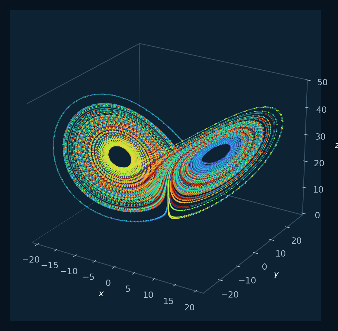
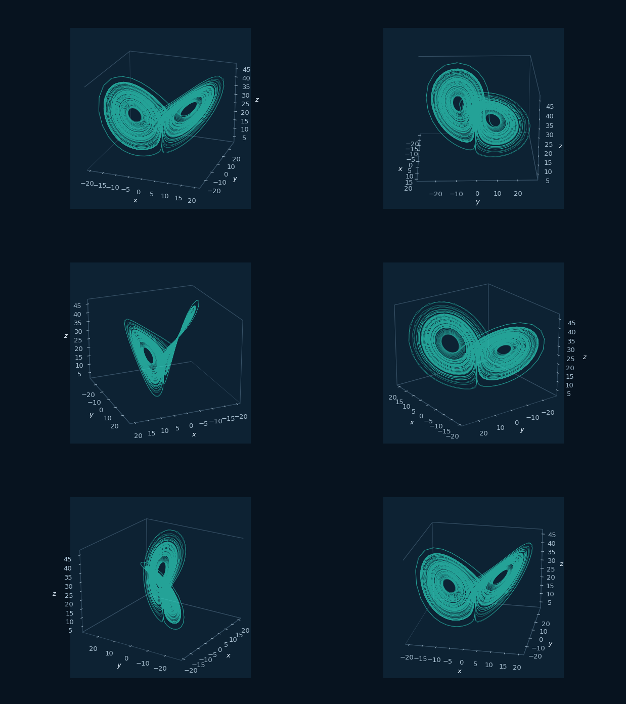
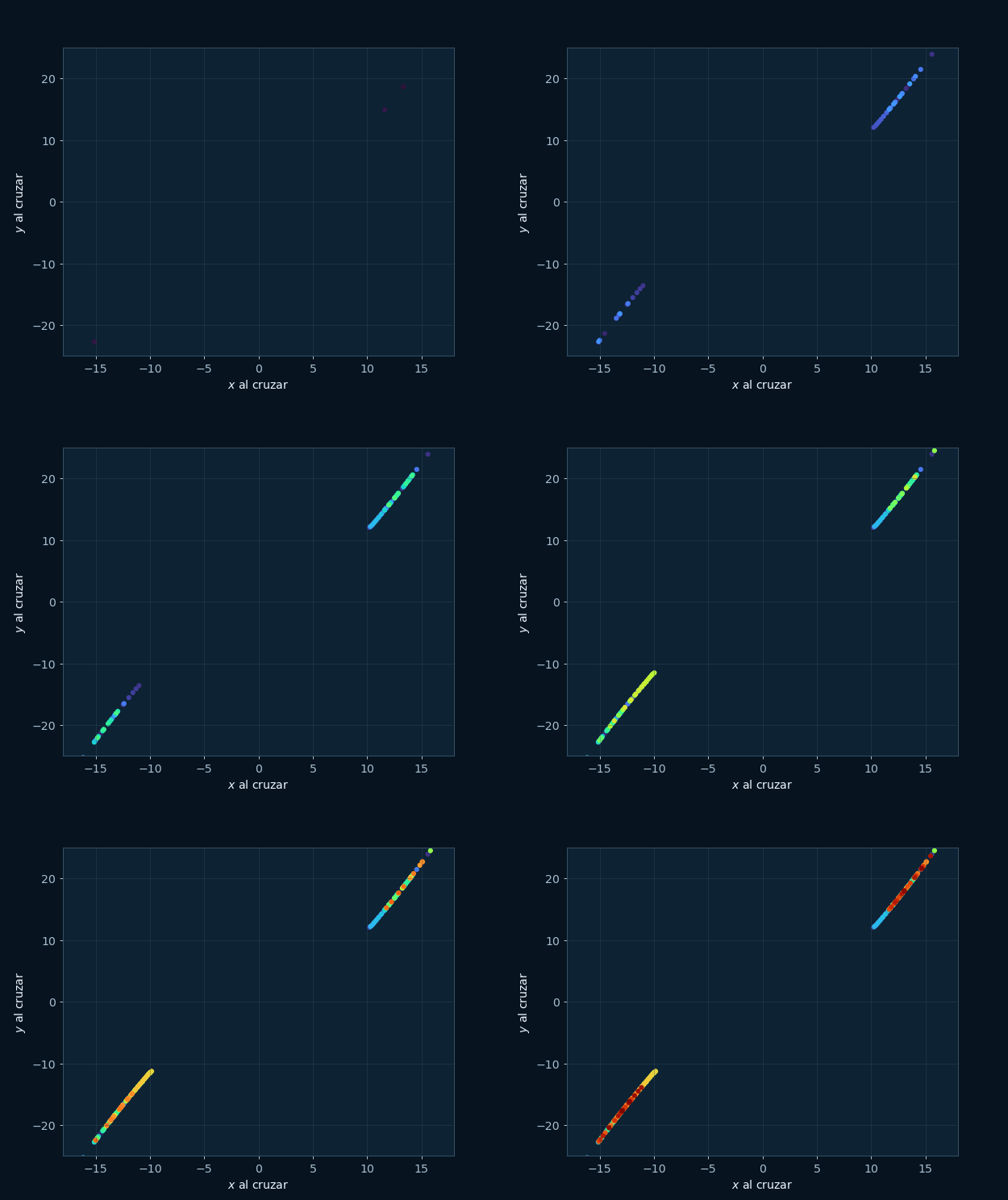
Simulación y proyecciones del sistema de Lorenz

Abre el flujo de trabajo de atractores 3D en Toolbox Chaos.
Elige Lorenz en el selector de sistemas.
Conserva los valores clásicos sigma = 10, rho = 28 y beta = 8/3, junto con el estado inicial (1, 1, 1).
Usa dt = 0.01, un tiempo total cercano a 40 y Runge–Kutta 4.
Ejecuta la simulación y gira el lienzo 3D para comprobar que ambos lóbulos de Lorenz sean visibles.
Cambia a los retratos de fase 2D y las series temporales para comparar las proyecciones y las trazas de las coordenadas antes de exportar.

Ecuaciones de Lorenz y geometría del espacio de fases

El sistema de Lorenz consta de tres ecuaciones diferenciales ordinarias estudiadas por Edward Lorenz en 1963 como un modelo simplificado de la convección atmosférica. En el régimen caótico clásico de parámetros, la trayectoria dibuja una forma semejante a una mariposa en el espacio de fases tridimensional.

Los ejes corresponden a las variables de estado x, y y z. La curva representa la historia del estado del sistema en el espacio de fases. Los dos lóbulos indican que la órbita visita repetidamente dos regiones, aunque el tiempo de alternancia es irregular.

Interpreta la gráfica 3D junto con las series temporales y las proyecciones 2D. La vista 3D muestra la geometría; x(t), y(t) y z(t) muestran la evolución temporal; y los retratos 2D revelan cómo se pliegan y retornan los pares de variables.

Parámetros que modifican la trayectoria

rho: al cambiar rho, Lorenz puede pasar de equilibrios estables a alternancias entre lóbulos y movimiento caótico.
Condición inicial: dos inicios cercanos pueden seguir recorridos parecidos brevemente y después separarse en el régimen caótico.
Tamaño de paso: un dt demasiado grande puede causar divergencia numérica o una trayectoria artificial.
Tiempo total: un intervalo demasiado corto muestra principalmente el transitorio; ventanas más largas revelan la geometría del atractor.
Proyección: las proyecciones x-y, x-z y y-z resaltan pliegues distintos, por lo que conviene examinar más de una vista.