Toolbox Chaos procedure
Three-Dimensional Trajectory Configuration
Generate a three-state trajectory, adjust its visual presentation, add coordinate-plane projections, and evaluate whether the geometry is numerically credible.
Question and result
Calculation performed
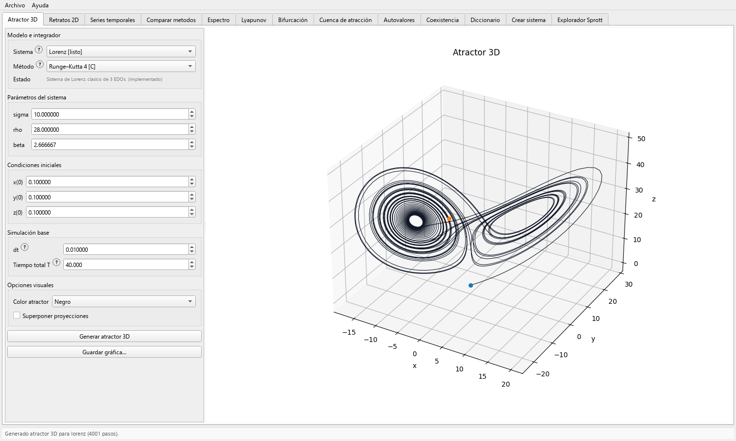
Use the 3D view as controlled geometric evidence with the projection and camera settings recorded.
Required configuration
- Select a catalog model whose displayed dimension is exactly three.
- Choose a justified parameter set, initial state, method, step size, and duration.
Panel and figure
Displayed quantities
Configuration and calculation
Control sequence
-
Select a compatible system
Choose a three-state entry such as Lorenz, Rössler, Chua, or Chen. The tab supports three-coordinate displays for the selected model.
Run the registered defaults once before changing the model parameters.
-
Set the simulation inputs
Enter the parameter vector and initial state in the labels shown by the interface. Select Euler, Heun, or RK4 and declare step and duration.
Use a smaller step for strongly curved or stiff-looking segments and a longer duration when the initial transient dominates the visible curve.
-
Choose the visual options
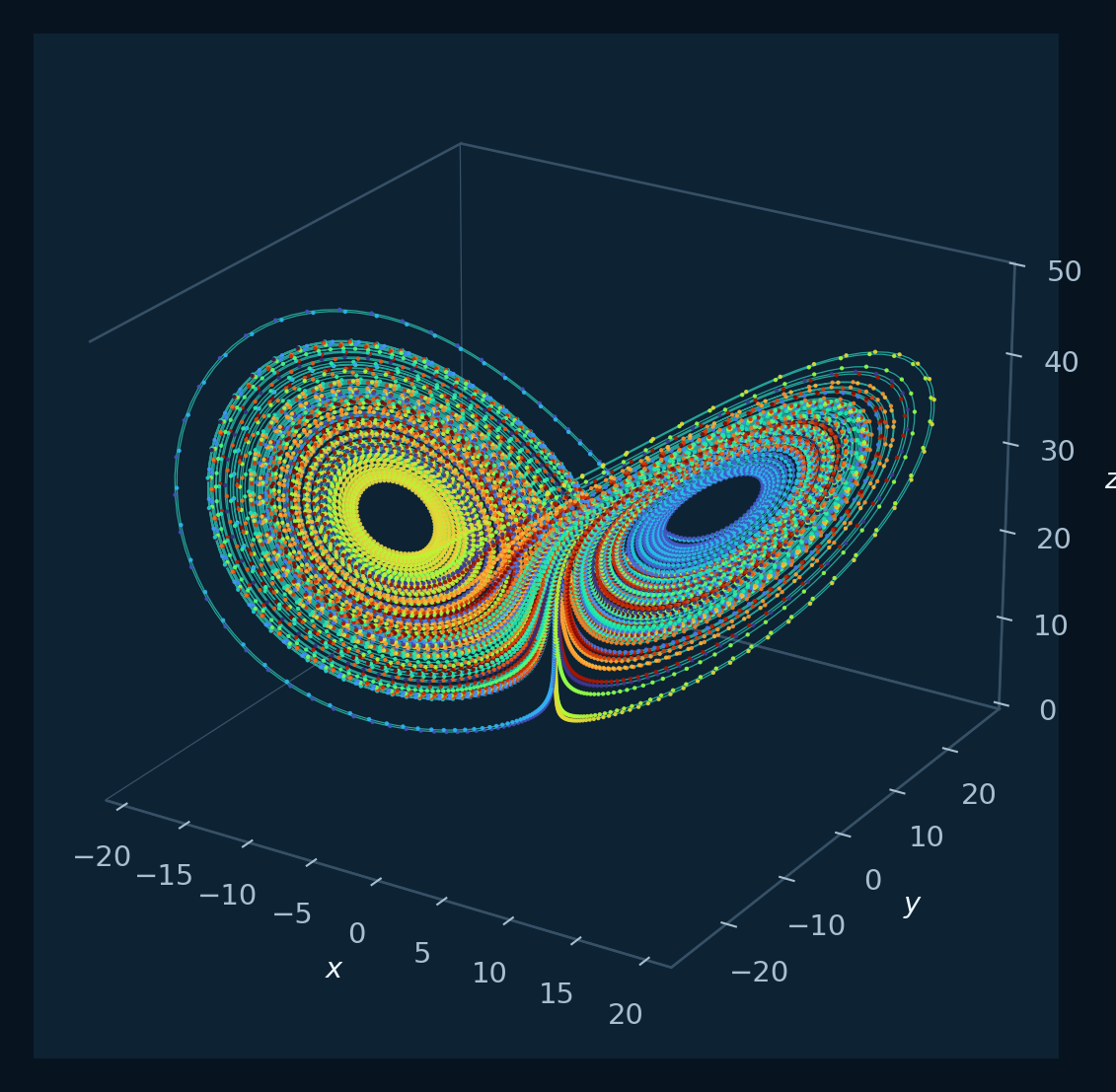
Set the attractor color independently of the equations. Enable Superponer proyecciones when coordinate-plane shadows will help connect the 3D curve to 2D portraits.
Compare two runs with common camera angles and axis scales, and record any declared visual variation.
-
Generate and rotate
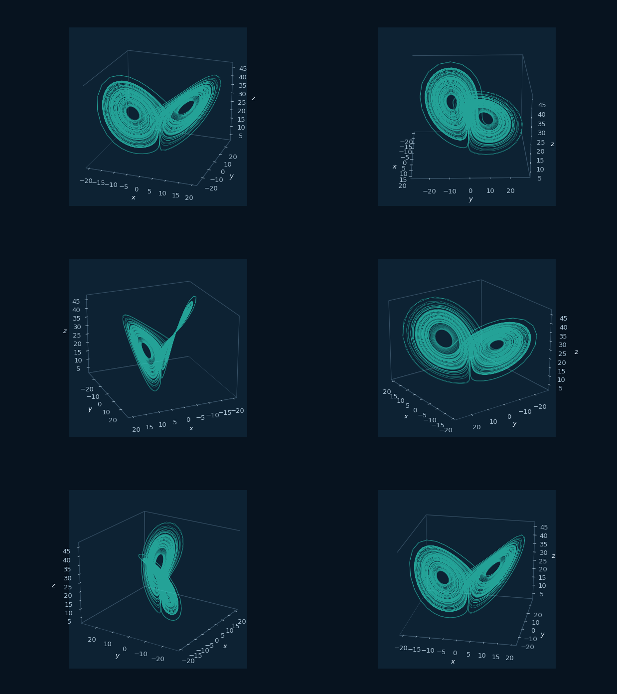
Press Generar atractor 3D, then rotate the canvas to check overlap, thin structures, symmetry, and regions hidden by the first viewpoint.
Inspect the early approach segment and identify it as the transient before examining recurrent geometry.
-
Test numerical stability
Repeat with half the step and compare the large-scale occupied region and lobe sequence across the sampled trajectories.
Repeat with a longer horizon and a nearby initial condition. Report whether the qualitative geometry persists and where it differs.
-
Save the figure
Use Guardar gráfica... to export at the GUI's publication-oriented resolution. Save a second view if one camera angle hides important structure.
Include variable names, parameter values, integration contract, and any transient handling in the figure caption or companion record.
Record
Computed data
- A finite three-dimensional state trajectory whose axes, parameters, initial state, and numerical resolution are known.
- Optional coordinate-plane projections that agree with separately generated pairwise portraits.
Scientific reading
Interpretation criteria
Dense recurrent-looking geometry suggests that the simulated orbit revisits a bounded region. Self-crossings in a 2D projection can arise from distinct points of the 3D trajectory.
Late trajectories from nearby starts may separate even when they occupy a similar region; this is why geometric agreement and pointwise agreement are different tests.
Files
Experiment record
- Save at least one view with readable axes and a reproducible camera orientation description.
- Record whether coordinate-plane projections were overlaid.
- Pair the 3D image with time series or 2D portraits from the same run.
Applications
Questions addressed by the calculation
- Communicating phase-space geometry in teaching and publications.
- Screening parameter regions before a systematic bifurcation or Lyapunov study.
- Comparing large-scale occupied regions under controlled parameter or initial-condition changes.
Scope
Evidence conditions
- The renderer may decimate a very long trajectory for responsive display; preserve the numerical contract: method, step, duration, initial state, parameters, and rendering settings.
- An invariant attracting set is assessed with declared numerical checks and the relevant mathematical analysis.
- Hidden-attractor basins are studied through the dedicated Hidden Attractors FO engine.