Lyapunov Diagnostics

Calculate Lyapunov exponents and visualize how small perturbations expand or contract in simulated systems.

Difficulty Level Intermediate

Question Do perturbations grow?

Question and result

Calculation performed

Estimate a finite-time Lyapunov spectrum for a compatible 3D flow under the tab's fixed RK4 QR–Benettin contract and decide whether the reported signs are numerically converged enough to support further study.

GUI tab

Lyapunov

Configuration and calculation

Control sequence

Select a supported flow and reproduce the same parameters and initial condition used for its trajectory.
Use the Lyapunov panel's own dt control with a conservative value, then set burn-in, final time, and the QR renormalization interval. The calculation uses fixed-step RK4 regardless of the general method selector displayed with the shared system controls.
Calculate the spectrum and inspect the convergence curves together with the final values.
Repeat with longer final time, adjusted burn-in, and a smaller dt; compare whether the signs and approximate values stabilize.

Record

Computed data

Three finite-time exponent estimates for a supported 3D flow and curves showing how those estimates evolve during accumulation.
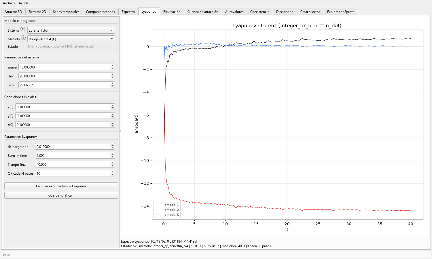
For the classical Lorenz case, a numerically stable pattern with one positive, one near-zero, and one negative direction after adequate refinement.

Scientific reading

Interpretation criteria

A stable positive maximal estimate supports sensitive dependence for the tested trajectory and numerical protocol; the near-zero and negative directions provide consistency information for a continuous flow.

Drifting curves, changing signs, or strong step dependence identify the controls that require further refinement before a scientific claim.

Files

Experiment record

Save the convergence figure together with the displayed final exponent values.
Record the system, ordered parameters, initial state, the fixed RK4 QR–Benettin algorithm, Lyapunov-panel dt, burn-in, final time, QR interval, software version, and every refinement run used in the interpretation.

Applications

Questions addressed by the calculation

Supporting sensitivity analysis after trajectory and transient inspection.
Comparing numerical convergence across parameters, time horizons, and integration steps.
Teaching local expansion, neutral flow direction, contraction, and finite-time uncertainty.

Scope

Evidence conditions

Finite-time exponents depend on trajectory, duration, transient removal, solver, and renormalization settings.
A short positive estimate motivates a convergence study that separates transients and numerical error from the measured rate.
This tab supplies finite-time Lyapunov evidence. Attraction, basin structure, uniqueness, and hidden-attractor localization require their dedicated analyses.

Logarithmic separation of two nearby trajectories in the Lorenz system — Titleless animation: two almost identical Lorenz trajectories initially separate at an approximately exponential rate. The early slope supplies a finite-time rate; later saturation only means that the distance has reached the attractor scale.

Separation of two Lorenz trajectories with a fit to the initial growth interval — Quantitative reading: on a logarithmic vertical axis, an approximately straight segment permits a local slope estimate. Fit before geometric saturation and repeat after refining the step, transient, and horizon.

Current Toolbox Chaos Lyapunov tab showing the Lorenz finite-time spectrum — Current interface: the Lorenz finite-time spectrum is displayed together with all convergence curves and the integration contract.

Finite-time Lyapunov procedure

Open the Lyapunov workflow in the toolbox.
Select the target flow and keep the same parameters used for the trajectory plot.
The Lyapunov calculation uses a fixed-step RK4 QR–Benettin algorithm. Set its dedicated dt conservatively; for Lorenz, dt = 0.01 is a practical first value. This calculation follows its dedicated RK4 contract.
Use a burn-in interval before accumulating exponent estimates.
Run a long enough integration window before interpreting the maximal exponent.
Inspect the convergence plot together with the final number.
Report the spectrum as numerical evidence and add the convergence study required for a chaos claim.

Perturbation growth and finite-time estimates

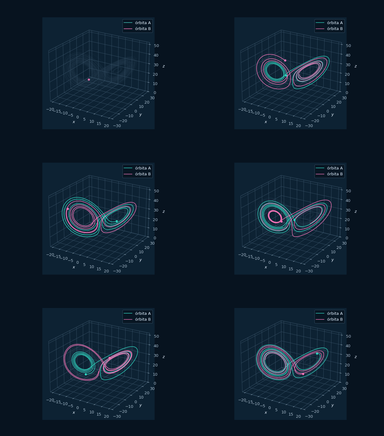
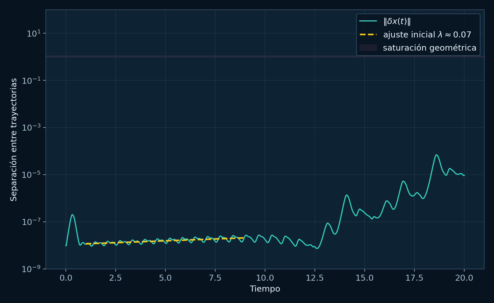
Lyapunov exponents measure average exponential rates of separation or contraction of nearby states in phase space. The number of exponents matches the system dimension. A positive maximal exponent is numerical evidence of sensitive dependence on initial conditions.

For a three-dimensional continuous flow, a typical chaotic spectrum has one positive exponent, one exponent close to zero, and one negative exponent. The near-zero direction corresponds to motion along the trajectory itself; the negative direction records contraction.

The convergence curves matter because finite-time estimates can drift. A student should ask whether the estimates stabilize when burn-in, final time, and integration step are refined.

The numerical contract of this tab is integer-order QR–Benettin with a fixed RK4 integrator. Report the dedicated Lyapunov dt, burn-in, measurement time, and QR interval shown with the result, and identify the calculation as the dedicated QR–Benettin method.

Horizon, transient, and perturbation controls

Burn-in: too little burn-in lets startup behavior bias the exponent estimate.
Total time: short integrations can give the wrong sign or unstable values.
Step size: a large step can create artificial expansion or contraction.
Perturbation size: perturbations must stay small enough to approximate local tangent behavior.
Renormalization interval: if vectors are renormalized too rarely, they can overflow or collapse into one direction.
Initial condition: hidden transients or multistability can change the observed finite-time spectrum.