The toolbox supports a teaching sequence in which students connect definitions with reproducible graphics. The dictionary names the concepts, while this page identifies the evidence each diagnostic contributes and the additional checks required for broader claims.
Question and result
Calculation performed
Connect core dynamical-systems concepts with the specific Toolbox Chaos plots that illustrate them, and identify the evidence supported by each finite numerical view.
GUI tab
GUI tab
Diccionario as the reference, together with the scientific tab named by each concept
Configuration and calculation
Control sequence
Open Diccionario to identify the term and the mathematical question it addresses.
Choose the corresponding workspace, such as Atractor 3D, Retratos 2D, Series temporales, Bifurcación, Cuenca de atracción, Espectro, or Lyapunov.
Generate one controlled example with recorded equations, parameters, initial condition, method, step, duration, and transient treatment.
Read the relevant figure using the definition, graph explanation, and caution supplied in this guide.
Compare at least two complementary views before writing a conclusion, then complete the mini lab to connect geometry, time, frequency, parameter change, and sensitivity.
Record
Computed data
A concept-to-plot map that states the question answered by each visualization or diagnostic.
A small set of reproducible figures accompanied by cautious interpretations and explicit statements of what remains untested.
Scientific reading
Interpretation criteria
Trajectory, time-series, basin, bifurcation, spectrum, and Lyapunov views describe different properties; agreement among them is stronger evidence than visual complexity in one plot.
Definitions organize the investigation, while claims must remain proportional to the finite numerical experiment actually performed.
Files
Experiment record
Export the selected scientific figures from their originating tabs and identify each plot type in the caption.
Record the concept, system, equations or catalog entry, parameters, initial state, numerical method, dt or iteration count, duration, transient, projection, and diagnostic-specific settings.
Applications
Questions addressed by the calculation
Designing introductory laboratories and assessment activities in nonlinear dynamics.
Choosing complementary diagnostics for a research protocol before running a large parameter study.
Writing precise figure captions that distinguish geometry, temporal behavior, frequency content, sensitivity, and destination classes.
Scope
Evidence conditions
The dictionary and conceptual figures explain terminology; calculated or certified properties require their corresponding numerical or mathematical workflow.
Irregular appearance, broadband frequency content, and a short positive Lyapunov estimate require complementary chaos diagnostics.
Global invariance, uniqueness of destinations, and asymptotic behavior require evidence beyond finite visual exploration.
Equations and update rules
An equation or map supplies the update rule that defines a dynamical system.
Initial conditions
The initial condition launches the trajectory. In multistable systems it can change the final destination.
Trajectory representations
Each plot answers a specific question about geometry, destination, frequency, sensitivity, or parameter change.
Numerical evidence
Chaos is interpreted by combining diagnostics, trajectories, and convergence checks.
The GIF loads only when requested.
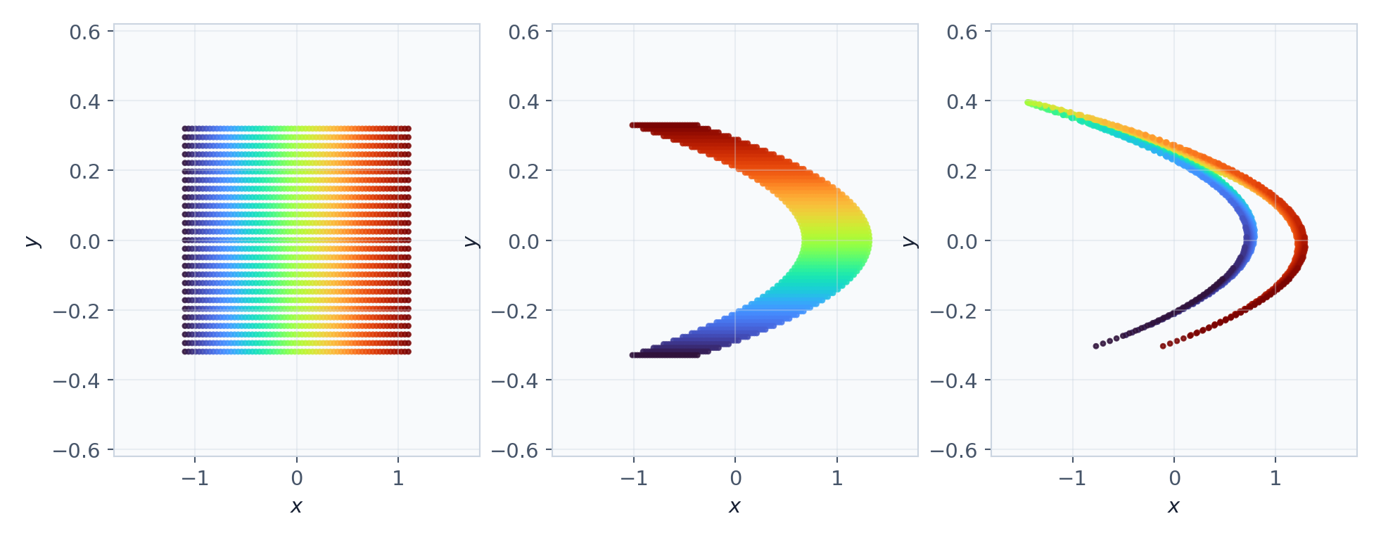
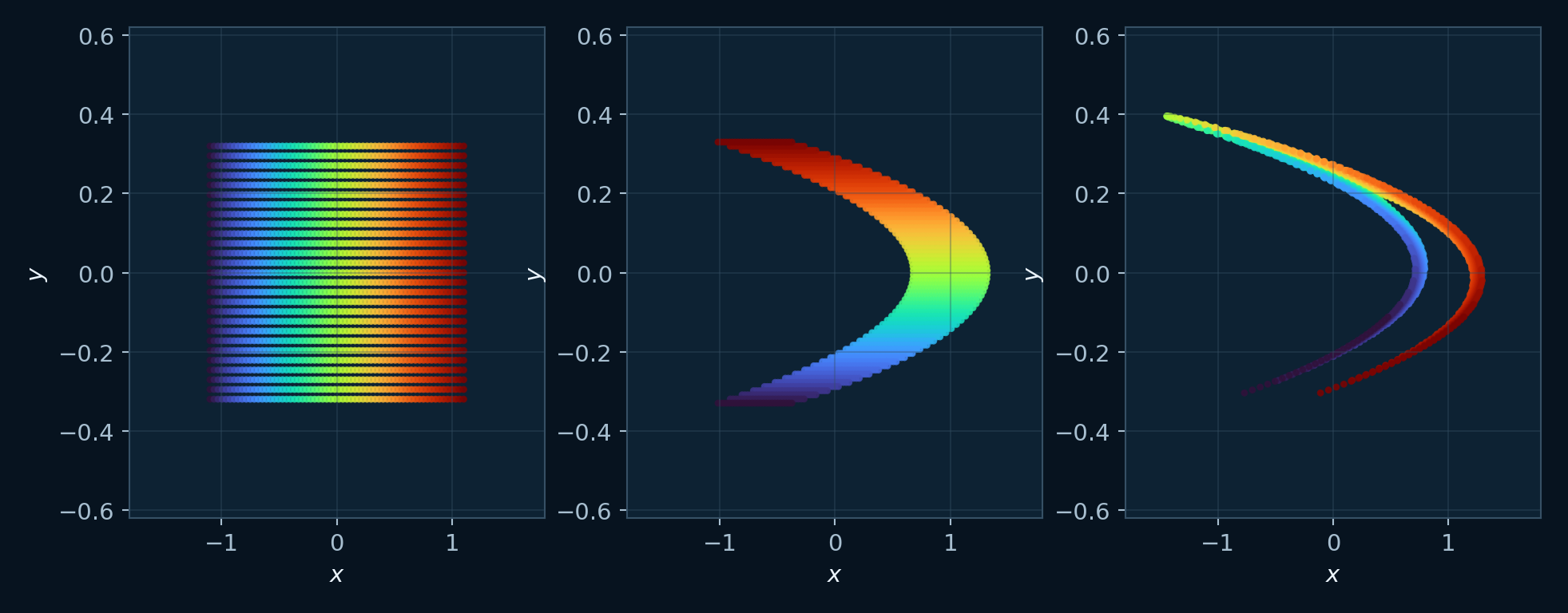
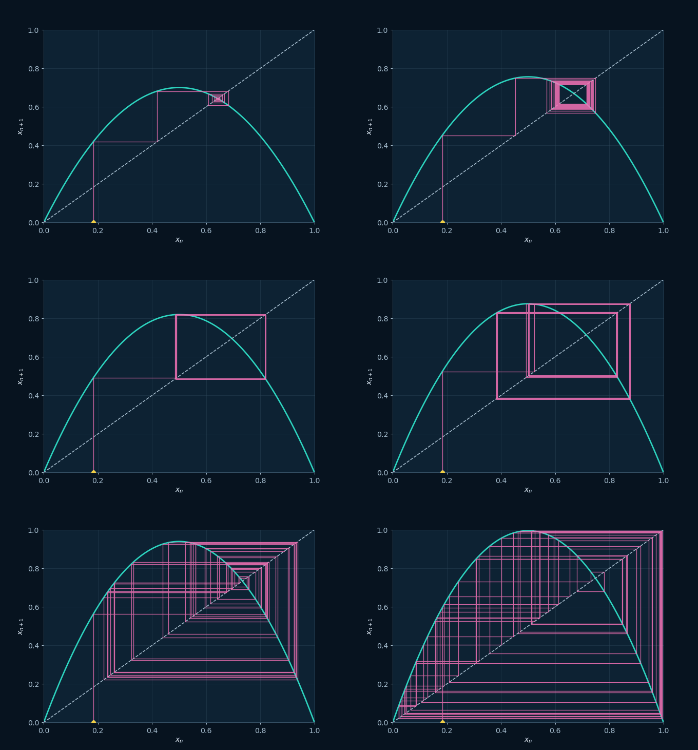
The panels isolate stretching and folding in a deterministic map. Nearby states are elongated, folded, and returned to the same bounded region; the on-demand sequence makes this geometric mechanism visible step by step.
What makes a system chaotic?
Chaotic System
Definition: A chaotic system is deterministic, nonlinear, bounded in the observed regime, and sensitive to initial conditions. Deterministic means that the same rule and the same initial condition reproduce the same trajectory. Sensitivity means that two extremely close initial conditions can separate measurably as time passes.
Watch for: Interpret irregular appearance with a suitable time step, simulation horizon, transient treatment, and readable projection.
The GIF loads only when requested.
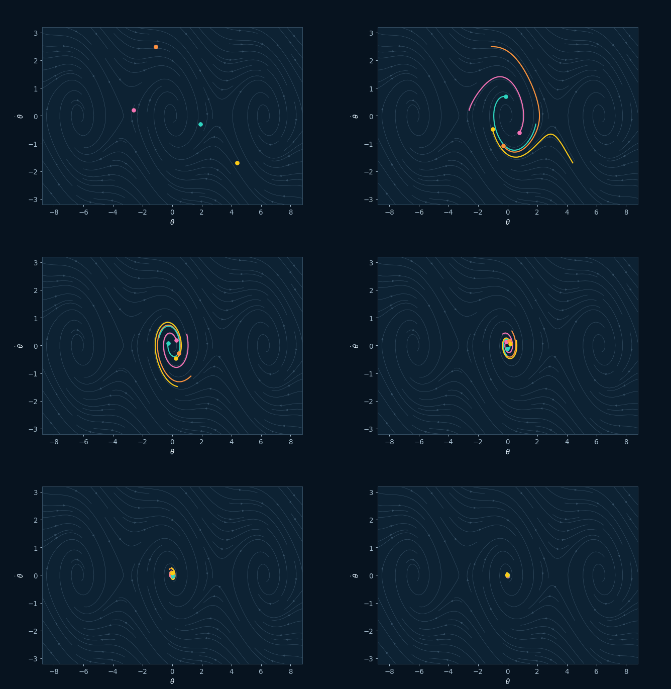
Every point is a possible state, the arrows encode the update rule, and the curve records the order in which one initial state evolves. The animation shows how the flow crosses the nullclines and turns a differential rule into motion.
What changes with time?
Dynamical System
Definition: A dynamical system is a rule for updating a state. In a continuous flow the rule is a differential equation, such as dx/dt = f(x,y,z). In a discrete map the rule advances by iterations, such as x(n+1)=F(x(n)).
Watch for: Record the displayed coordinates separately from the full system dimension; a high-dimensional model may be shown through two or three coordinates.
The GIF loads only when requested.
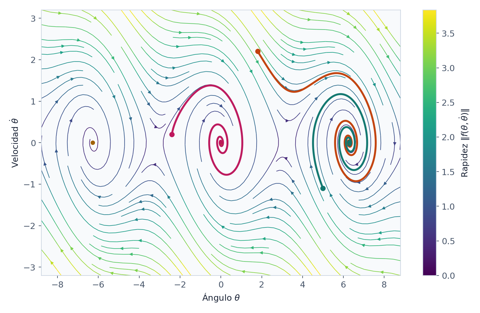
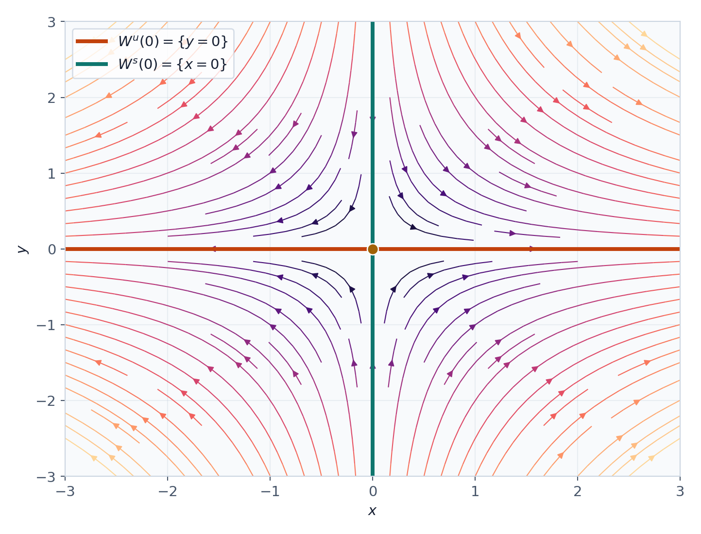
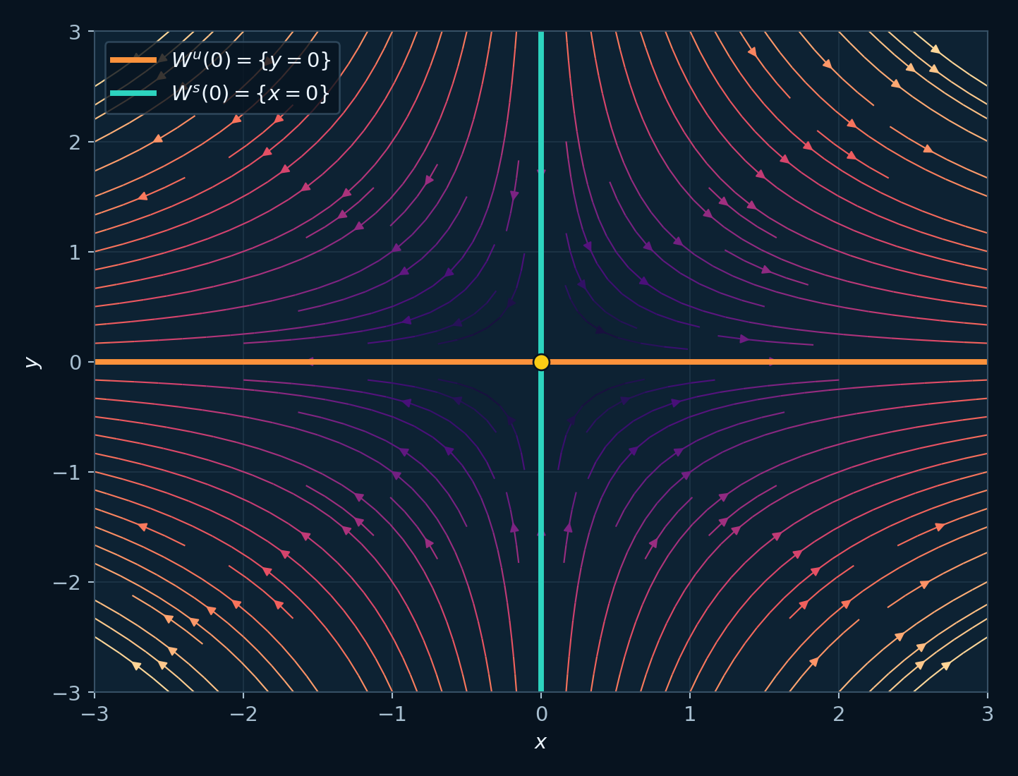
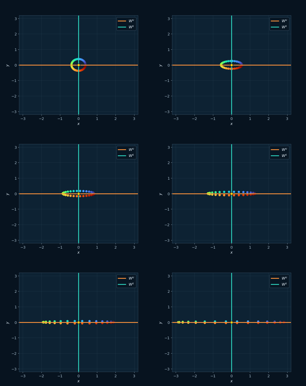
The portrait shows trajectories organized by the stable and unstable directions of a saddle. Moving points make time ordering explicit while the coordinate axes represent state variables.
Where does the motion live?
Phase Diagrams and Trajectories
Definition: A phase diagram plots state variables against each other. A 2D portrait can show x and y, while a 3D portrait can show x, y, and z. The plot emphasizes the geometry of motion in state space.
Watch for: A 2D projection can create apparent crossings. Use additional projections to recover depth and identify the relevant structure.
The GIF loads only when requested.
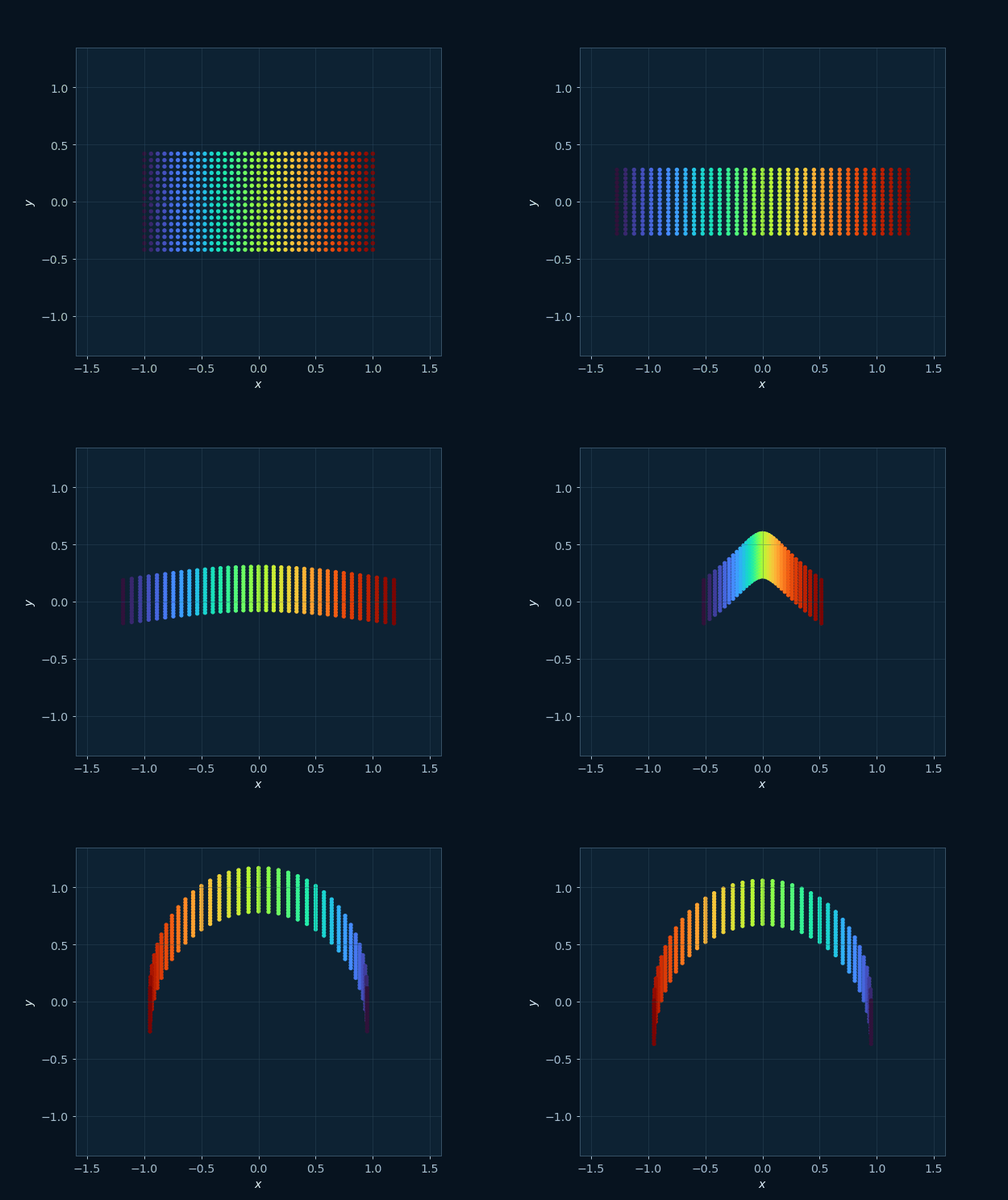
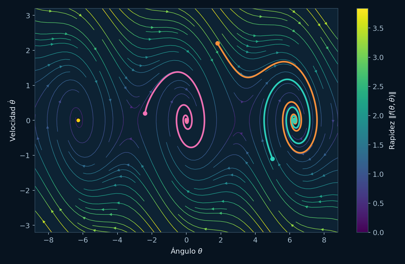
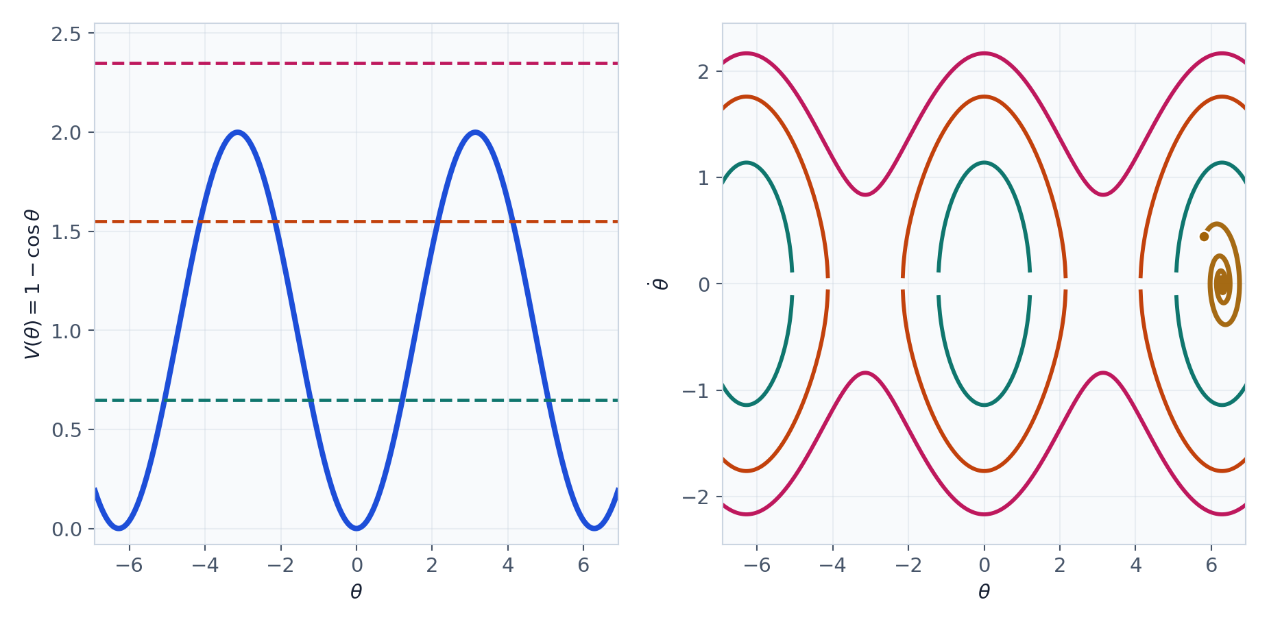
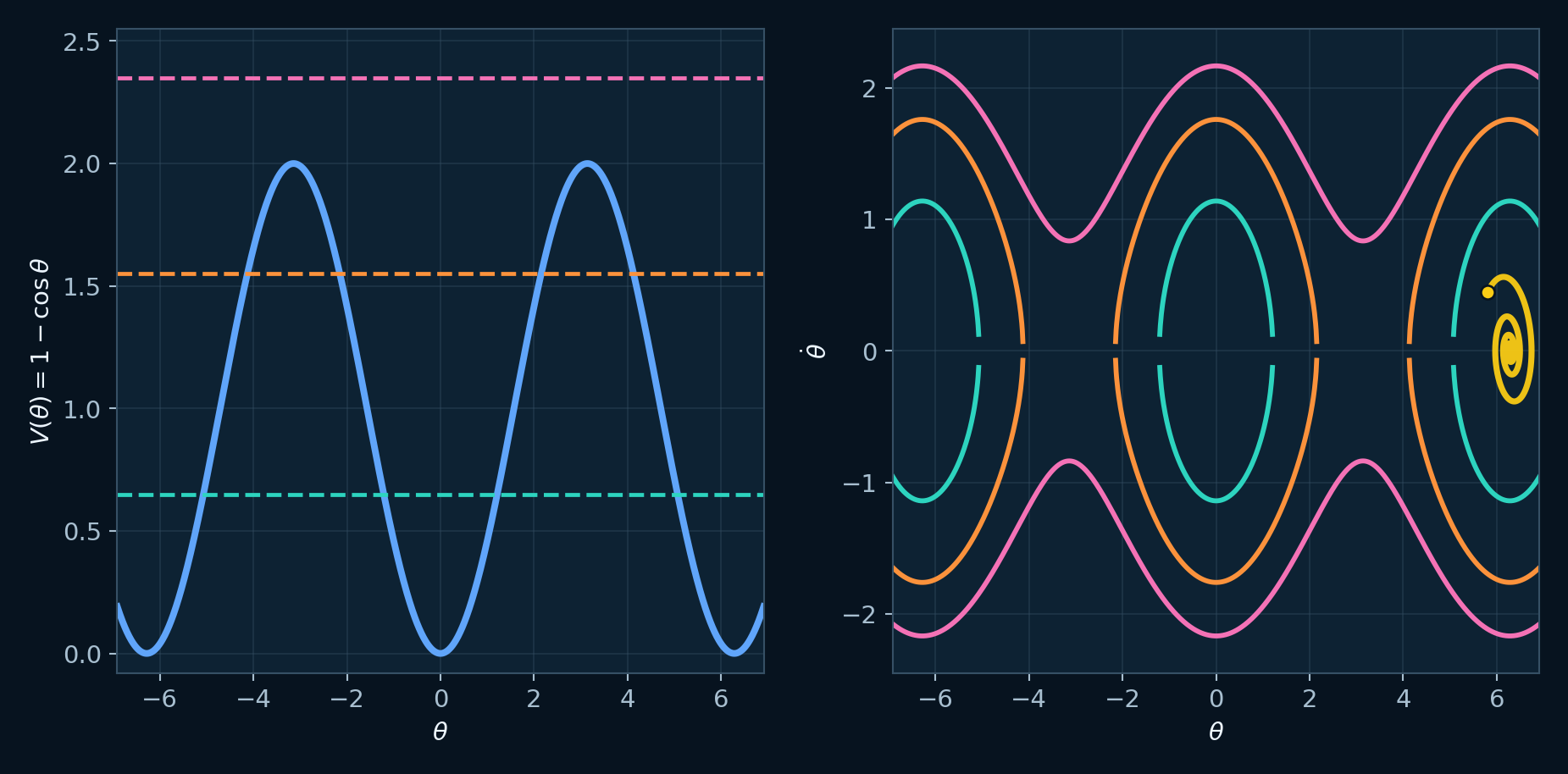
The potential-energy panel and the angle-velocity portrait describe the same pendulum from complementary viewpoints. Closed curves represent oscillations, while the separatrix divides oscillation from rotation.
Evidence from multiple projections
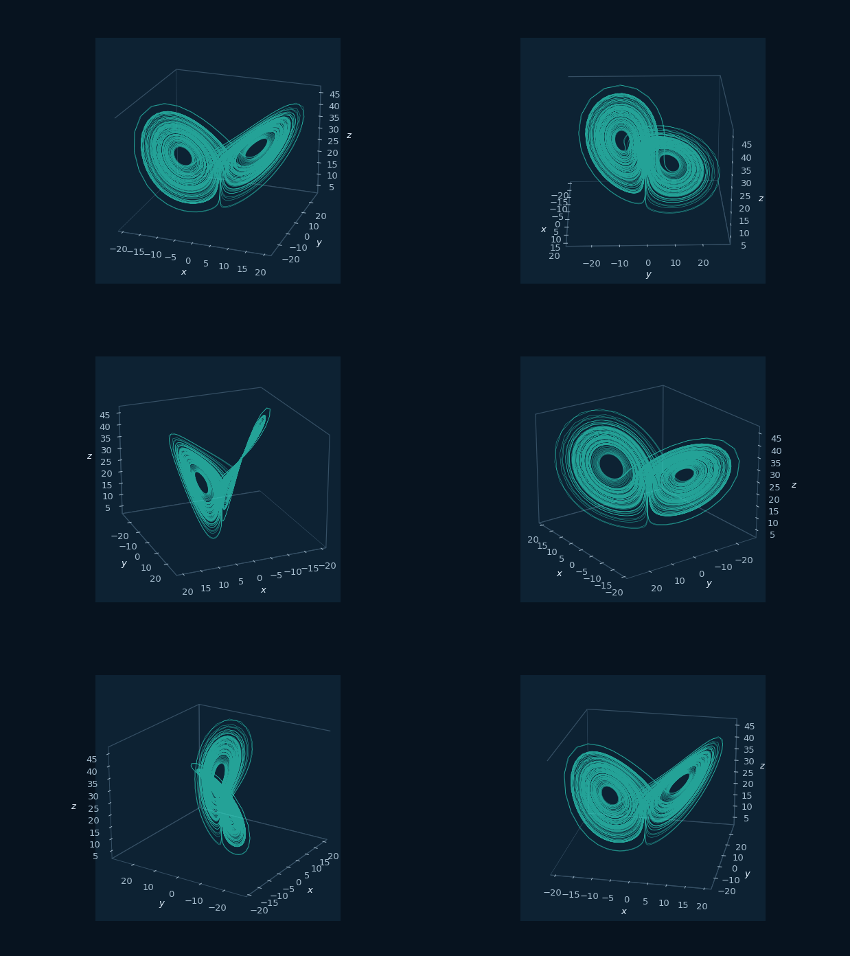
Separate 2D Phase Portraits
Definition: A 2D phase portrait is a projection of the state-space trajectory onto two selected variables. It simplifies the geometry so local folds, loops, and symmetries are easier to inspect.
Watch for: A projection presents the same trajectory through a selected set of coordinates.
The GIF loads only when requested.
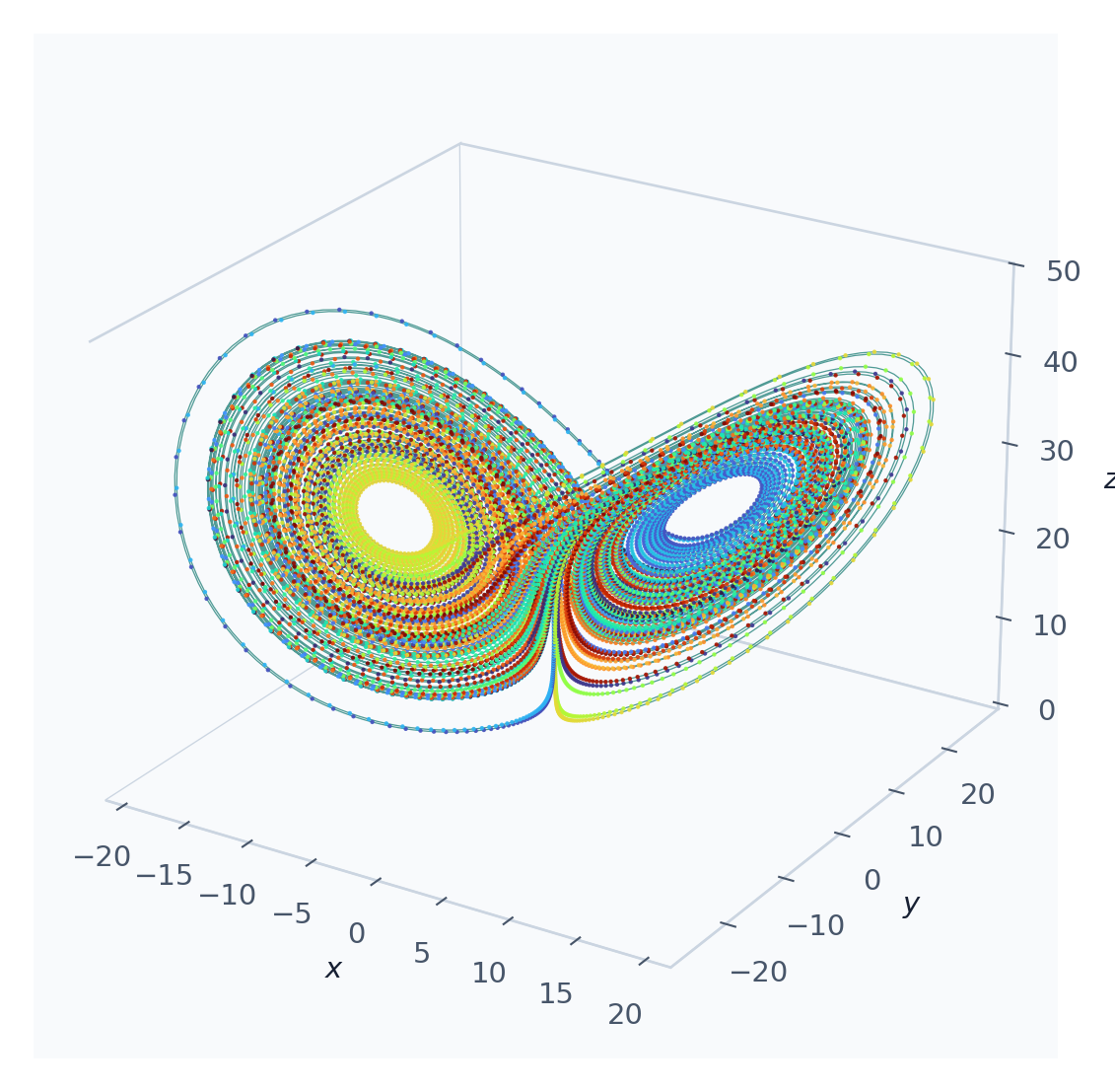
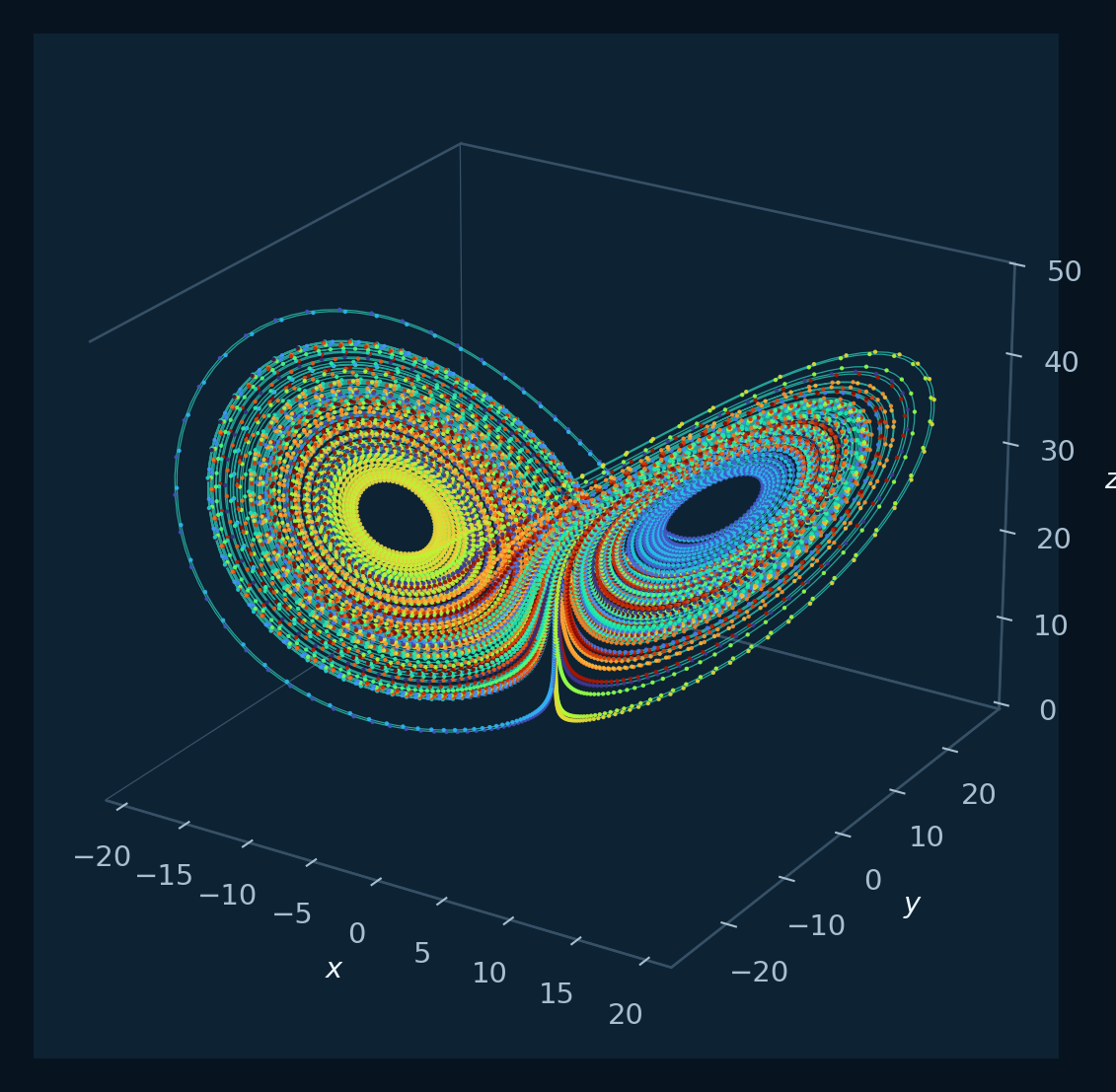
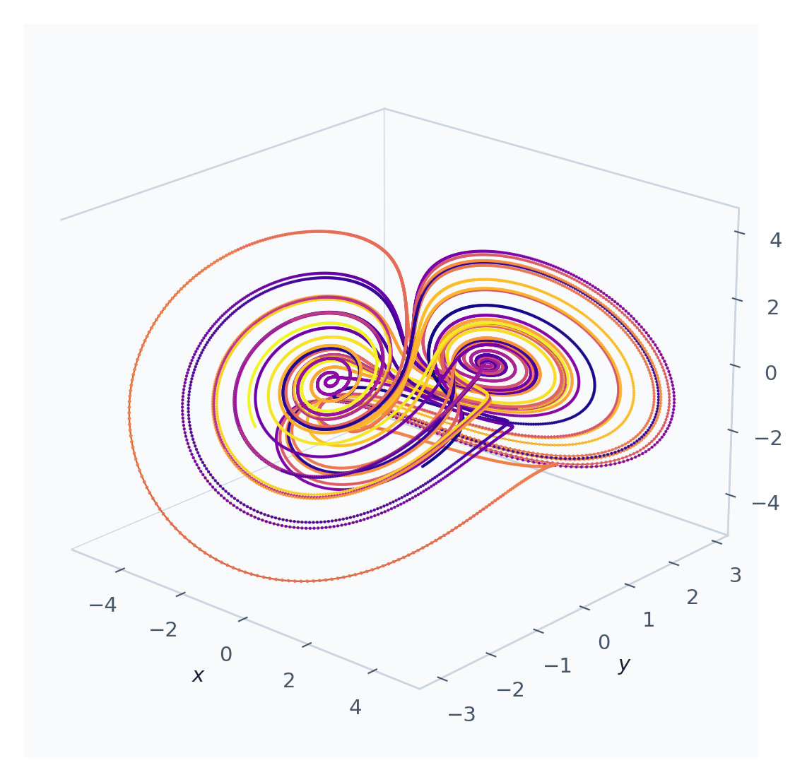
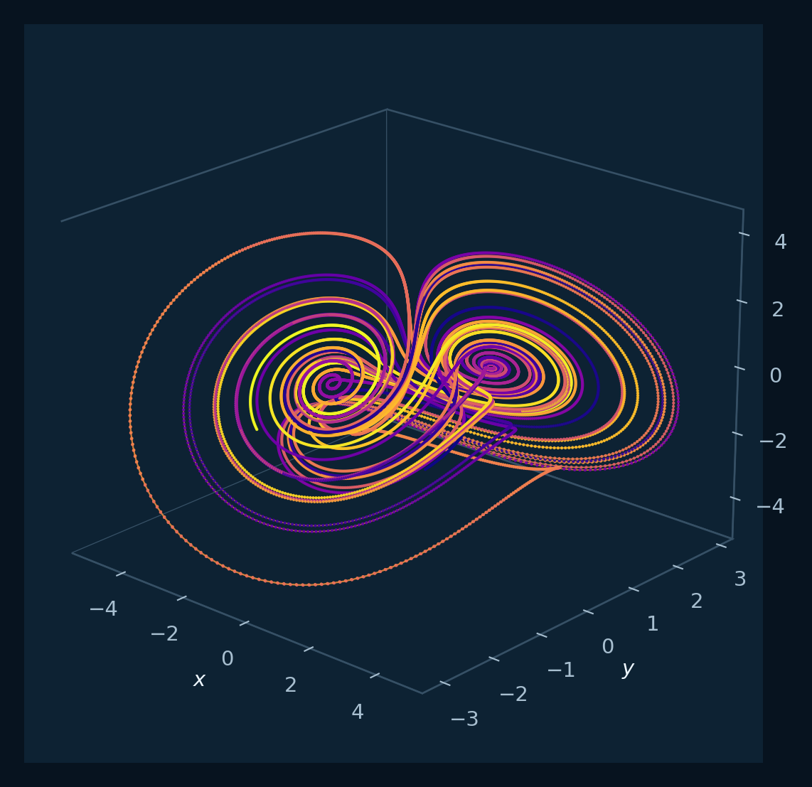
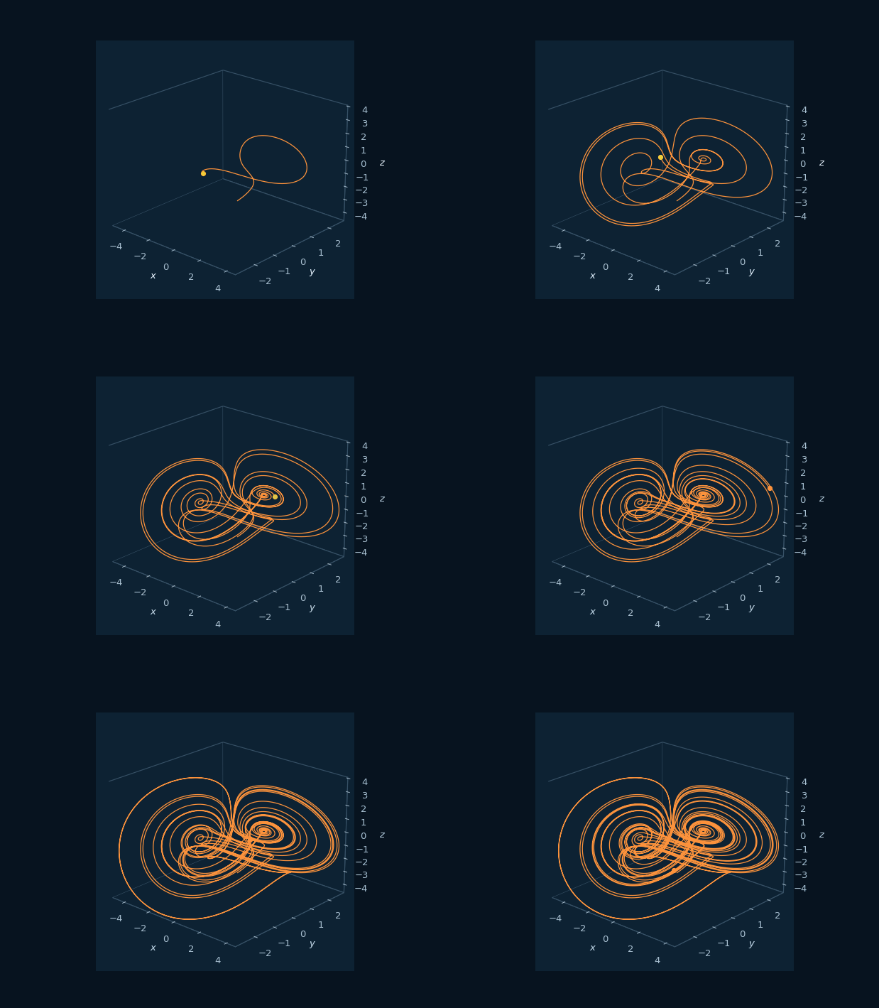
The classical Lorenz orbit repeatedly visits two lobes in an irregular order while remaining bounded. The rotating animation shows the folded 3D structure.
Where does the trajectory go after transients?
Attractor
Definition: An attractor is the set approached by a family of trajectories after initial transient behavior. It can be a fixed point, a limit cycle, a torus, a chaotic set, or another invariant structure.
Watch for: A two-lobed figure contributes geometric evidence alongside time series, bifurcation behavior, spectra, and Lyapunov estimates.
The GIF loads only when requested.
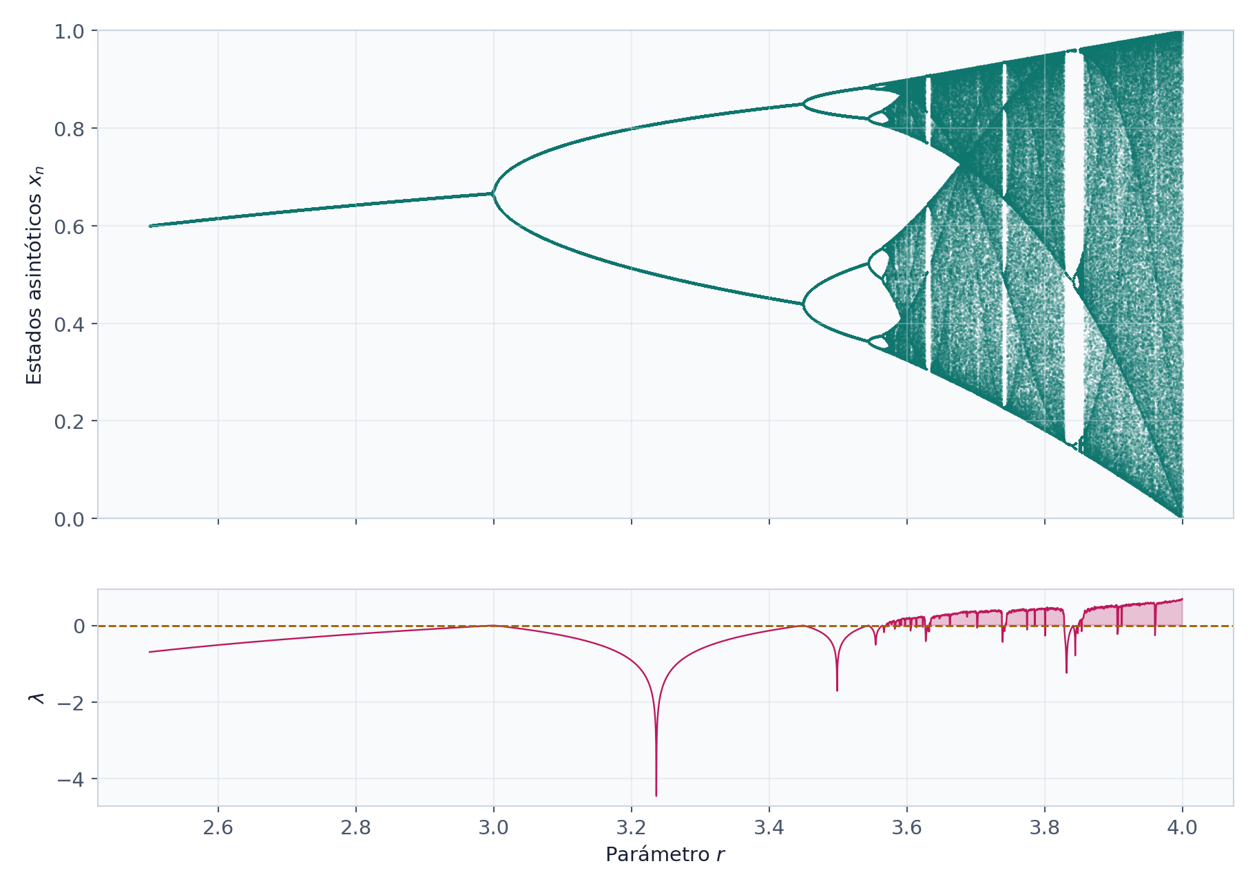
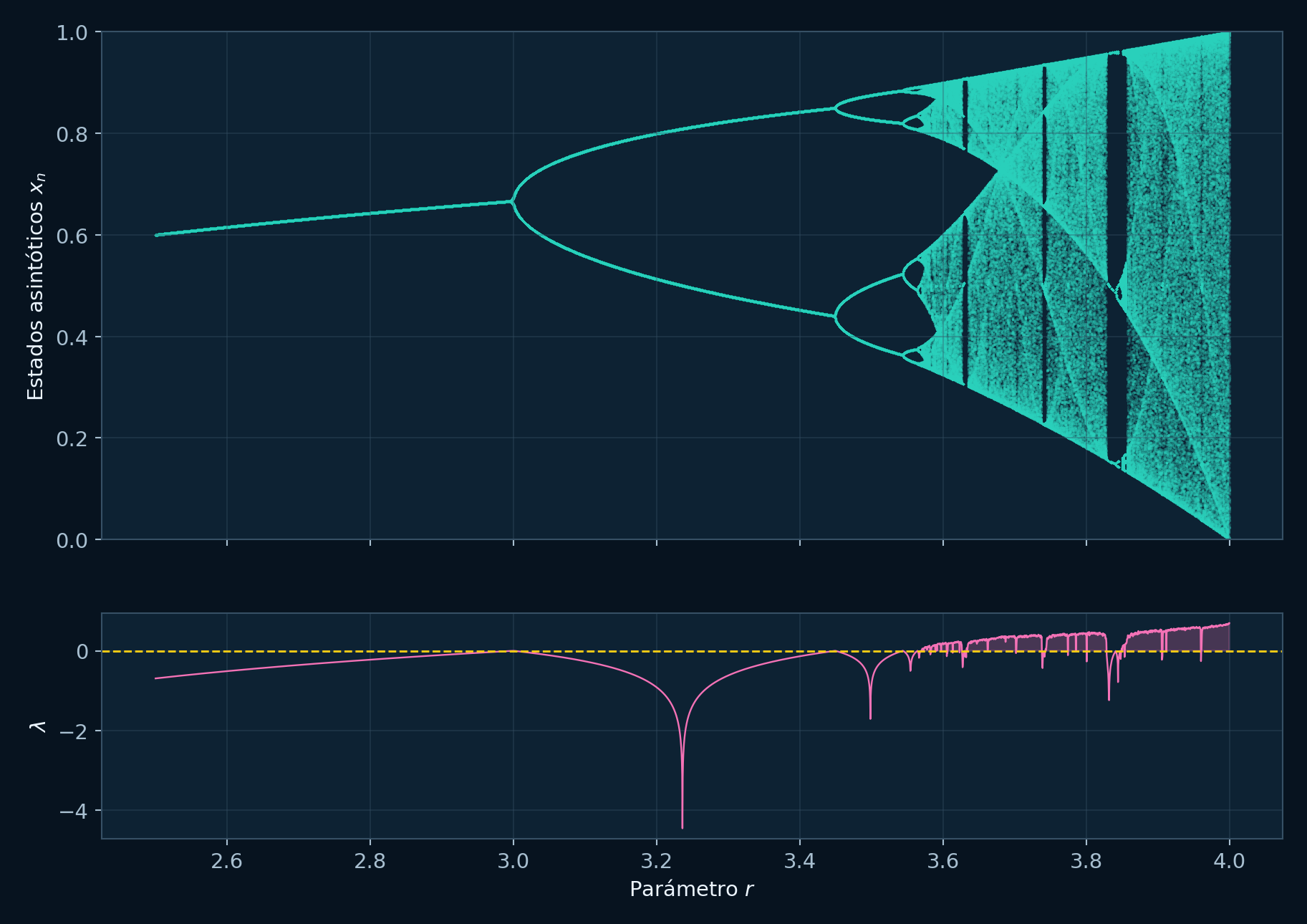
Each column corresponds to one parameter value of the logistic map. Retained iterates show the long-term values after transients: one branch, split branches, periodic windows, and dense bands reveal qualitative changes. The animation follows the iteration at one selected parameter.
What changes when a parameter changes?
Bifurcation Diagram
Definition: A bifurcation occurs when a small change in a control parameter changes the qualitative behavior of the system. Equilibria can lose stability, cycles can appear, periods can double, and chaotic bands can emerge.
Watch for: A sparse or tiny diagram is easy to misread. Increase the parameter samples, retained points, integration time, and figure size only after the interval has been located.
The GIF loads only when requested.
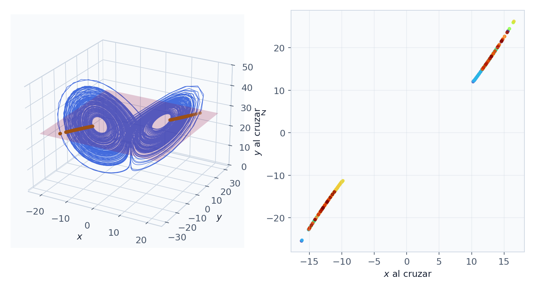
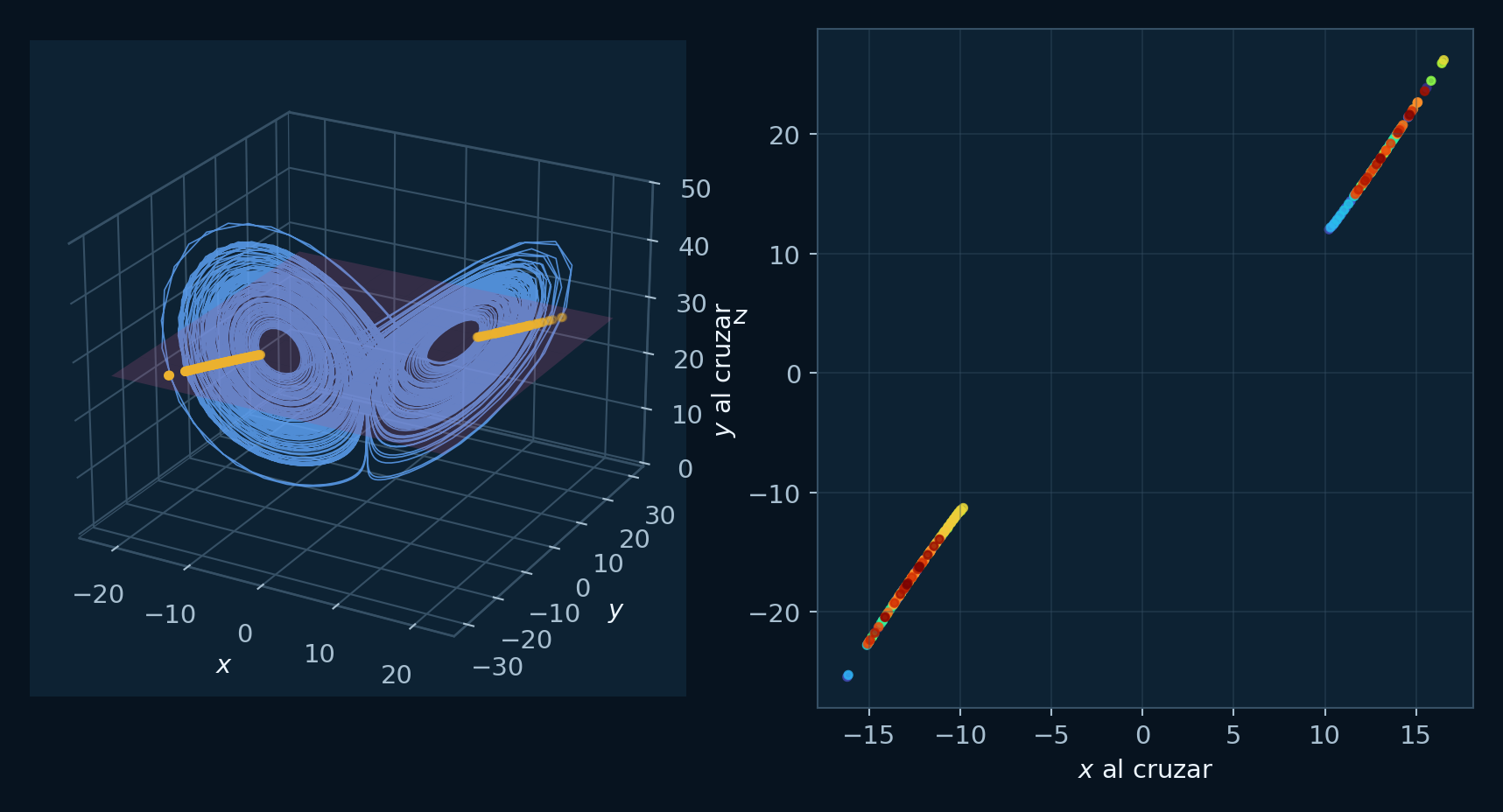
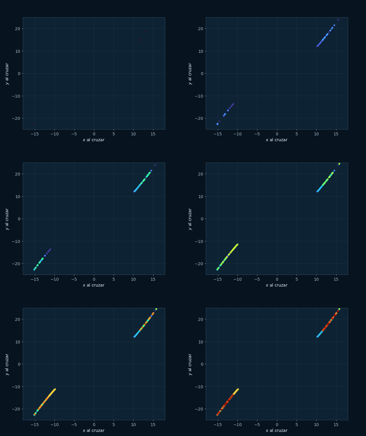
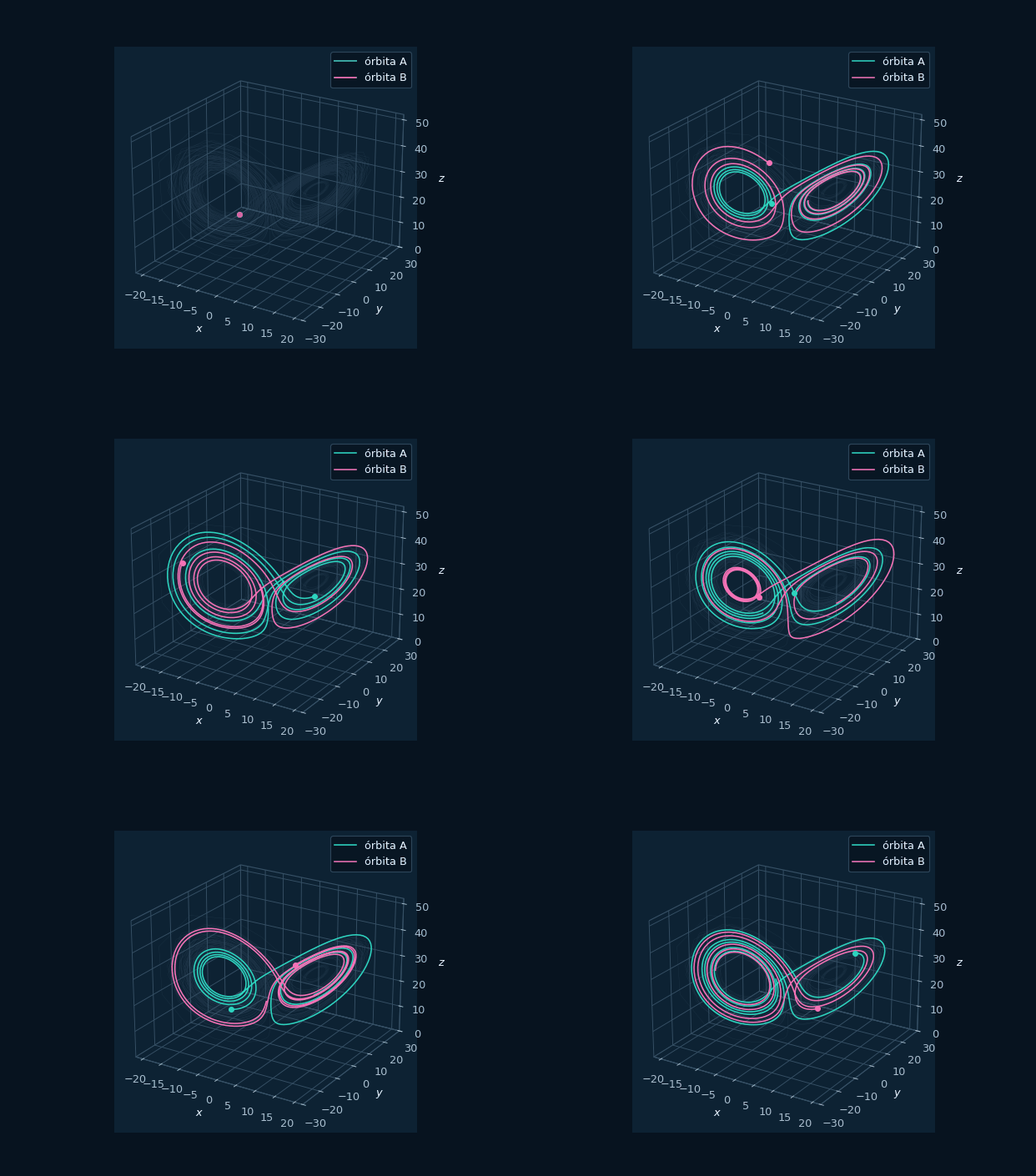
The figure shows the Lorenz trajectory, the section plane, and the crossing points. A periodic orbit would produce a small number of repeated points. A chaotic orbit produces a richer return structure.
How can a continuous flow be reduced to comparable returns?
Poincare Section
Definition: A Poincare section records intersections of a continuous trajectory with a chosen surface, often using a fixed crossing direction. It turns a flow into a sequence of return points.
Watch for: The section depends on the plane and crossing direction. A poorly chosen plane can show too few points or hide the behavior you meant to study.
The GIF loads only when requested.
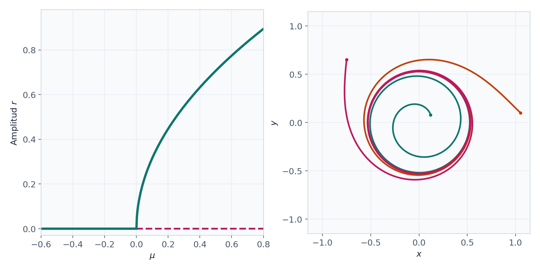
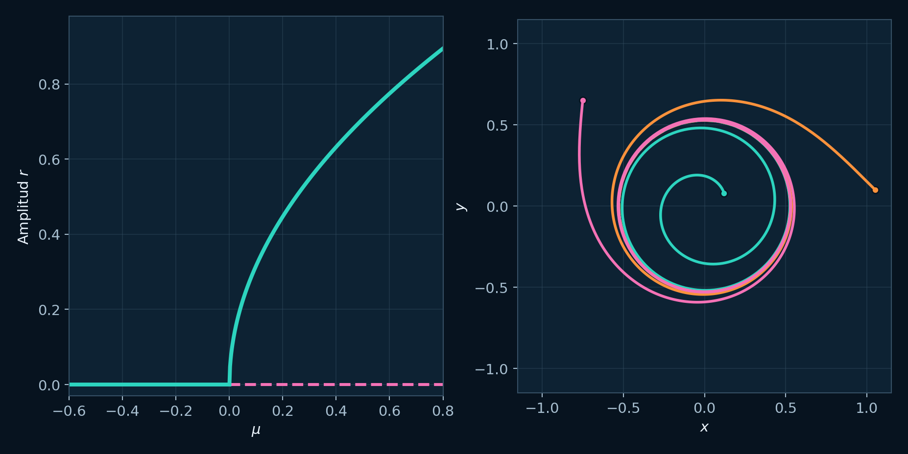
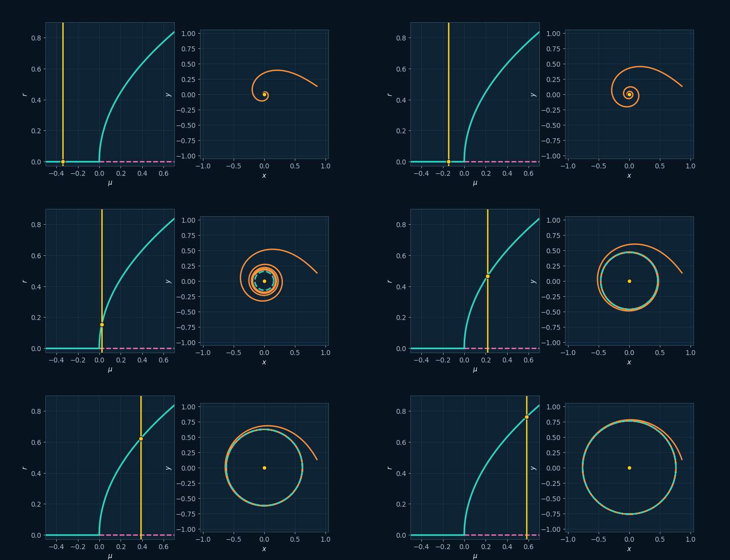
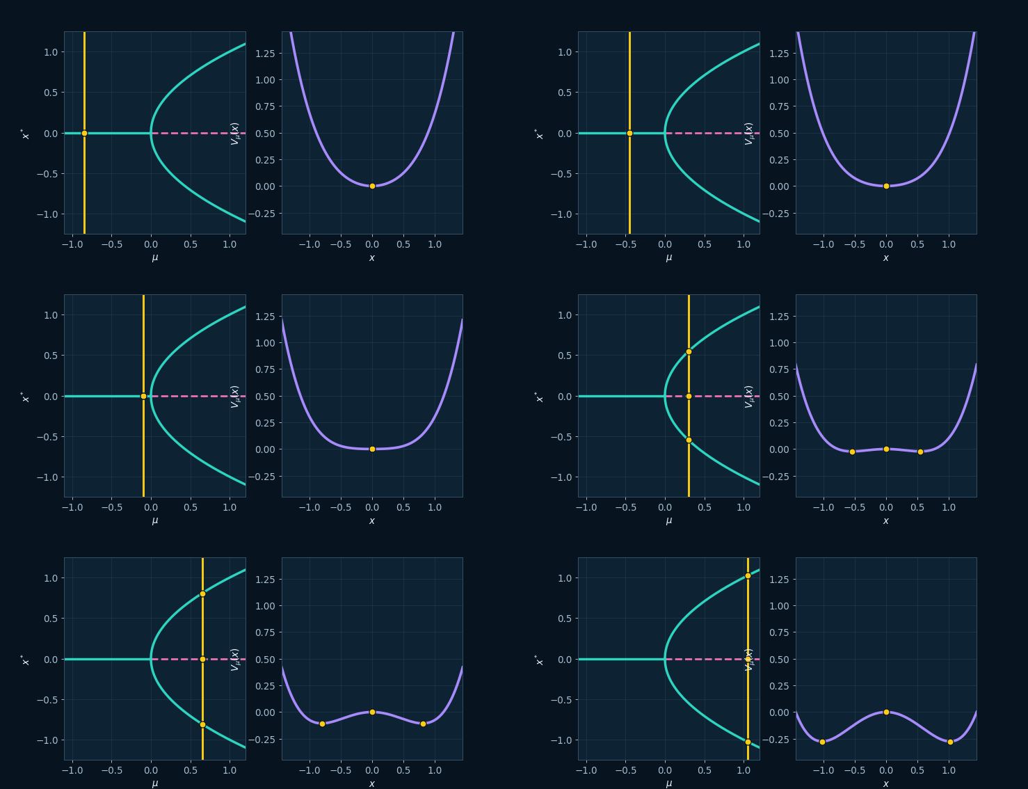
The conceptual figure contrasts a stable focus with the new oscillatory state and plots how the oscillation amplitude grows. It is a local mechanism for the birth of periodic motion.
How can an oscillation be born from an equilibrium?
Hopf Bifurcation
Definition: A Hopf bifurcation occurs when an equilibrium changes stability and a small oscillation appears or disappears around it. In a supercritical Hopf bifurcation, a stable limit cycle appears after the critical parameter is crossed.
Watch for: Hopf analysis describes the emergence of local oscillations. Chaos studies examine additional mechanisms such as period doubling, intermittency, crises, or global interactions.
The GIF loads only when requested.
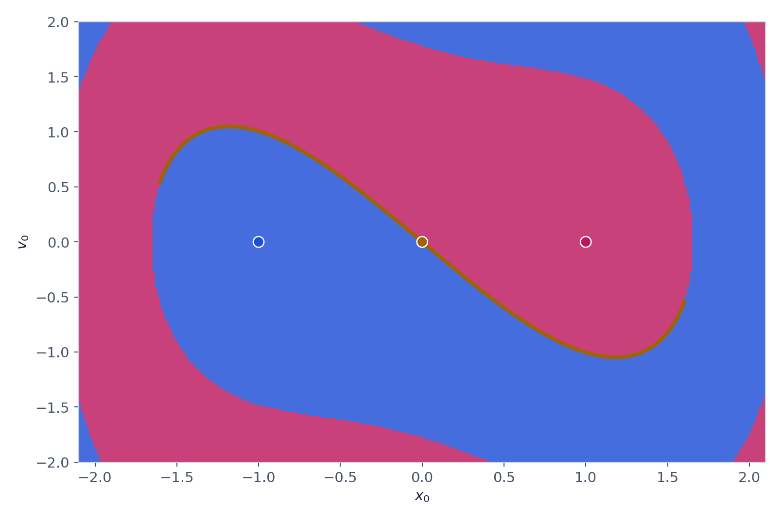
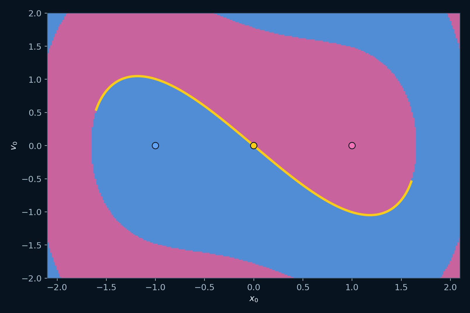
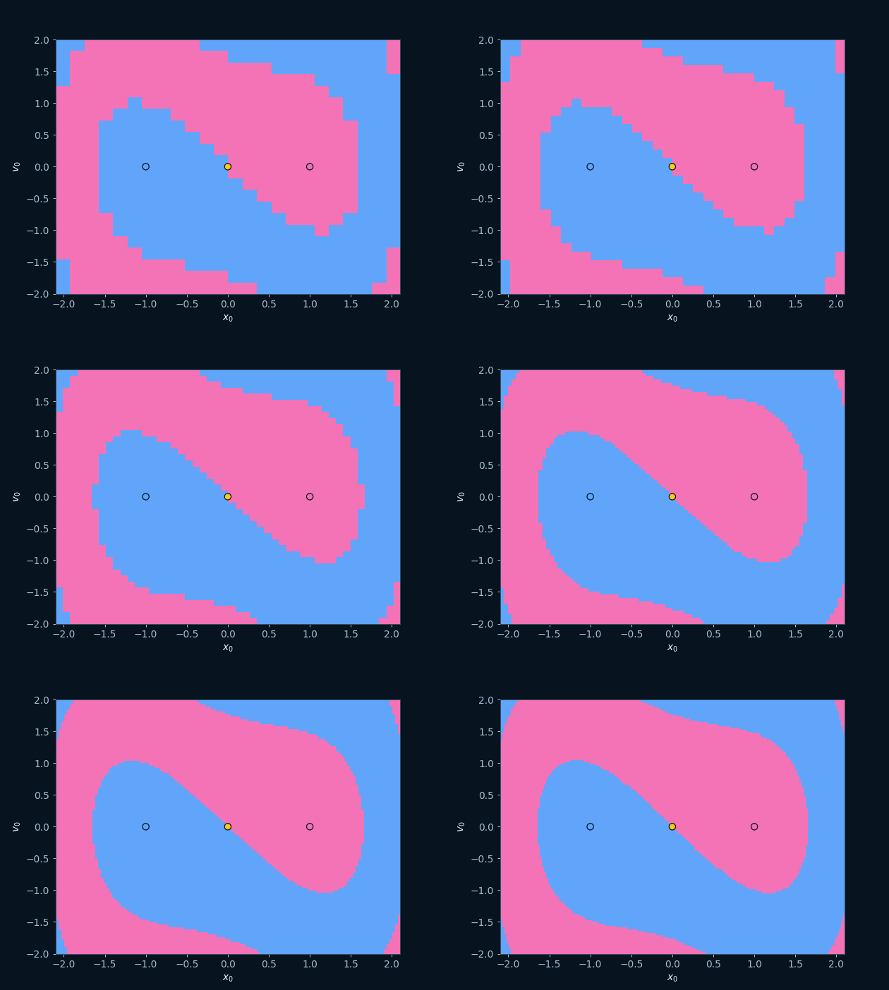
Each pixel is an initial condition and each color is a destination class. The animation refines the sampling grid so the boundary can be distinguished from coarse-pixel artifacts.
Which destination belongs to each initial condition?
Basins of Attraction
Definition: A basin of attraction is the set of initial conditions classified toward the same destination over a declared simulated horizon. When several computed destinations coexist, the sampled phase-space region is partitioned into colors.
Watch for: A basin classifies many initial conditions, whereas a coexistence plot compares selected starts.
The GIF loads only when requested.
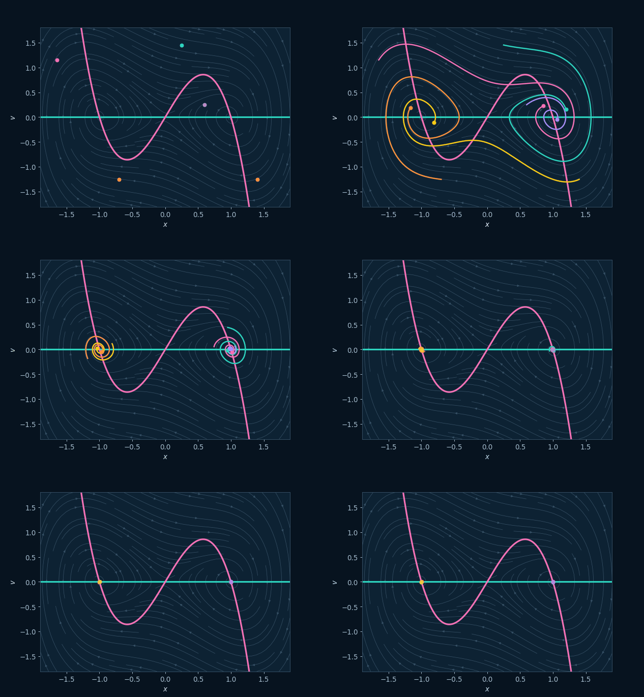
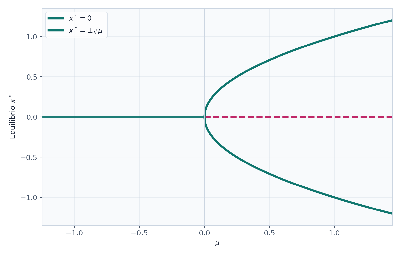
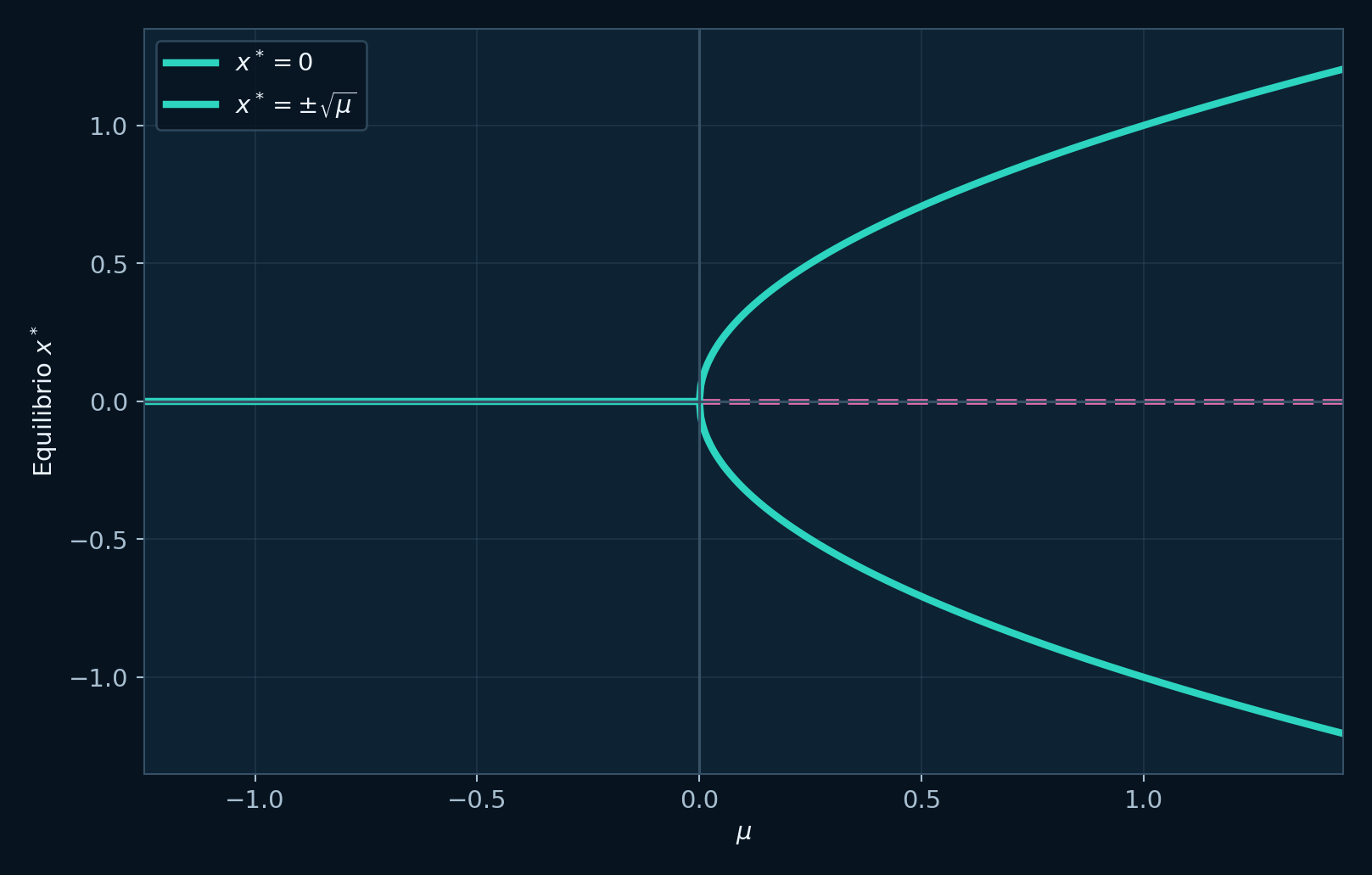
The pitchfork diagram provides a clean local model of coexistence: after the critical parameter, two stable branches are available under the same rule and parameter. The animation changes only the parameter and shows how the possible destinations are created.
Coexisting destinations under fixed parameters
Coexisting Attractors
Definition: Coexistence means that the equations and parameters remain fixed, but sampled initial conditions reach different computed destinations over the declared horizon. Multistability requires additional evidence that those destinations remain stable under small perturbations.
Watch for: Coexistence can involve equilibria or attractors. This Lorenz example contains two stable fixed points.
The GIF loads only when requested.
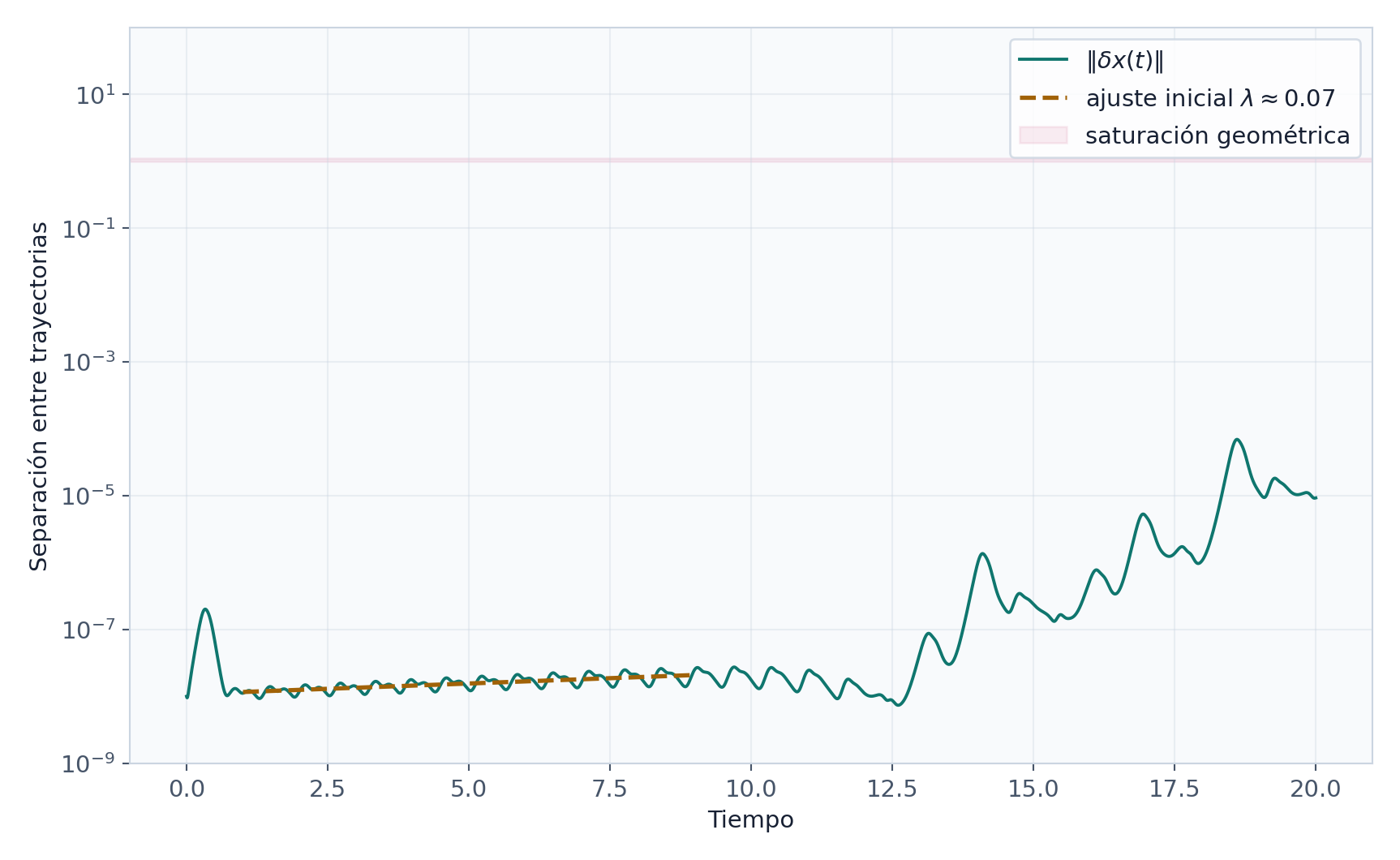
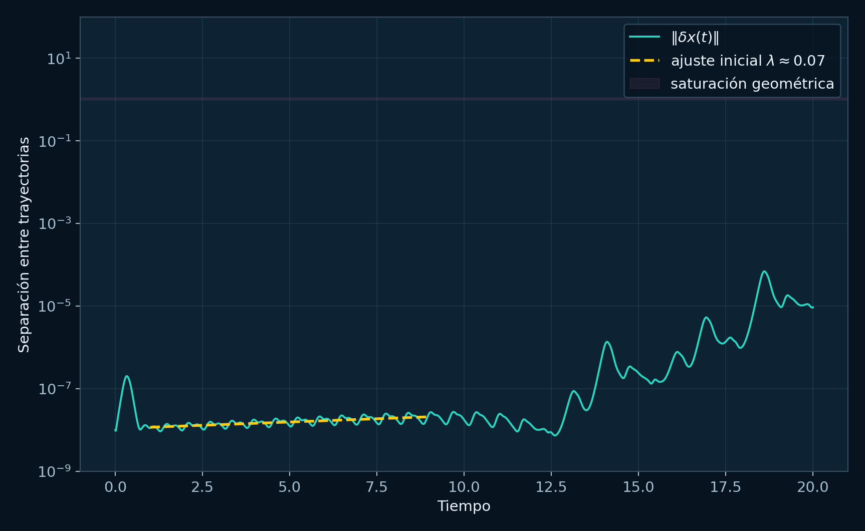
The near-linear interval in the logarithm of trajectory separation estimates the average expansion rate. The animation compares two nearby Lorenz starts; their visible separation introduces the quantity, while a converged exponent supplies the numerical estimate.
How is sensitivity to initial conditions measured?
Lyapunov Exponents
Definition: Lyapunov exponents measure average rates of expansion or contraction of small perturbations. A positive exponent indicates that nearby trajectories separate exponentially on average.
Watch for: Finite-time estimates can drift. Interpret the sign and magnitude only after checking transient removal, integration time, step size, and convergence.
The GIF loads only when requested.
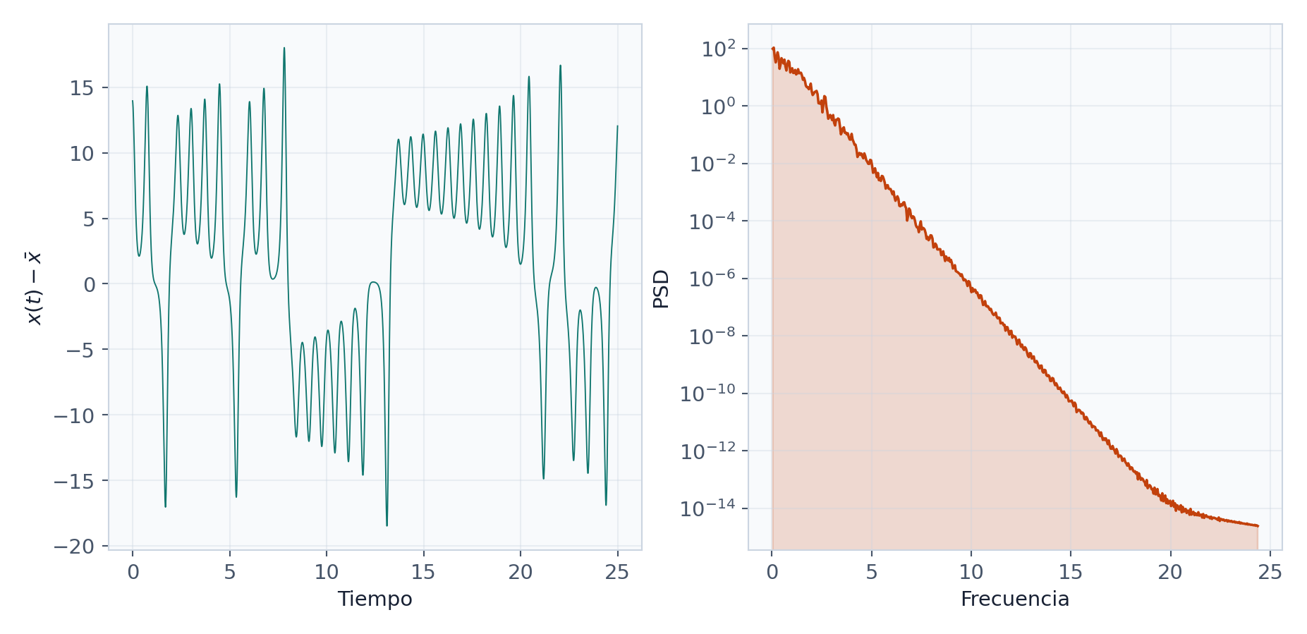
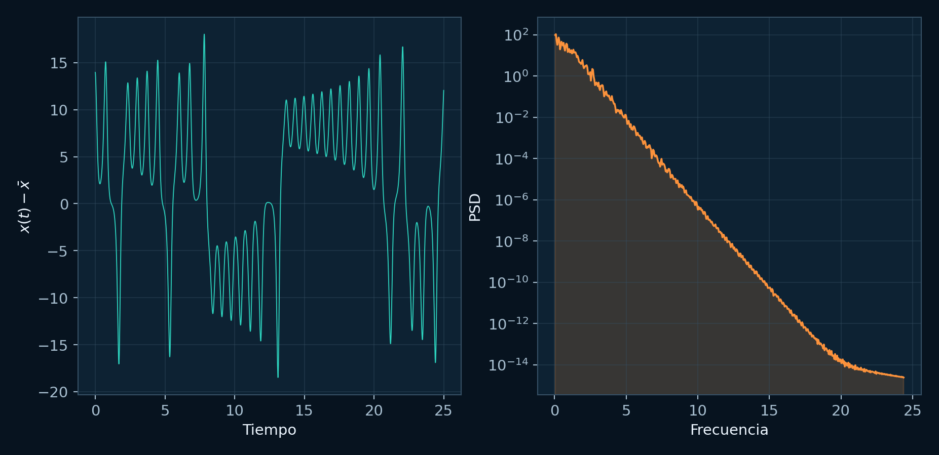
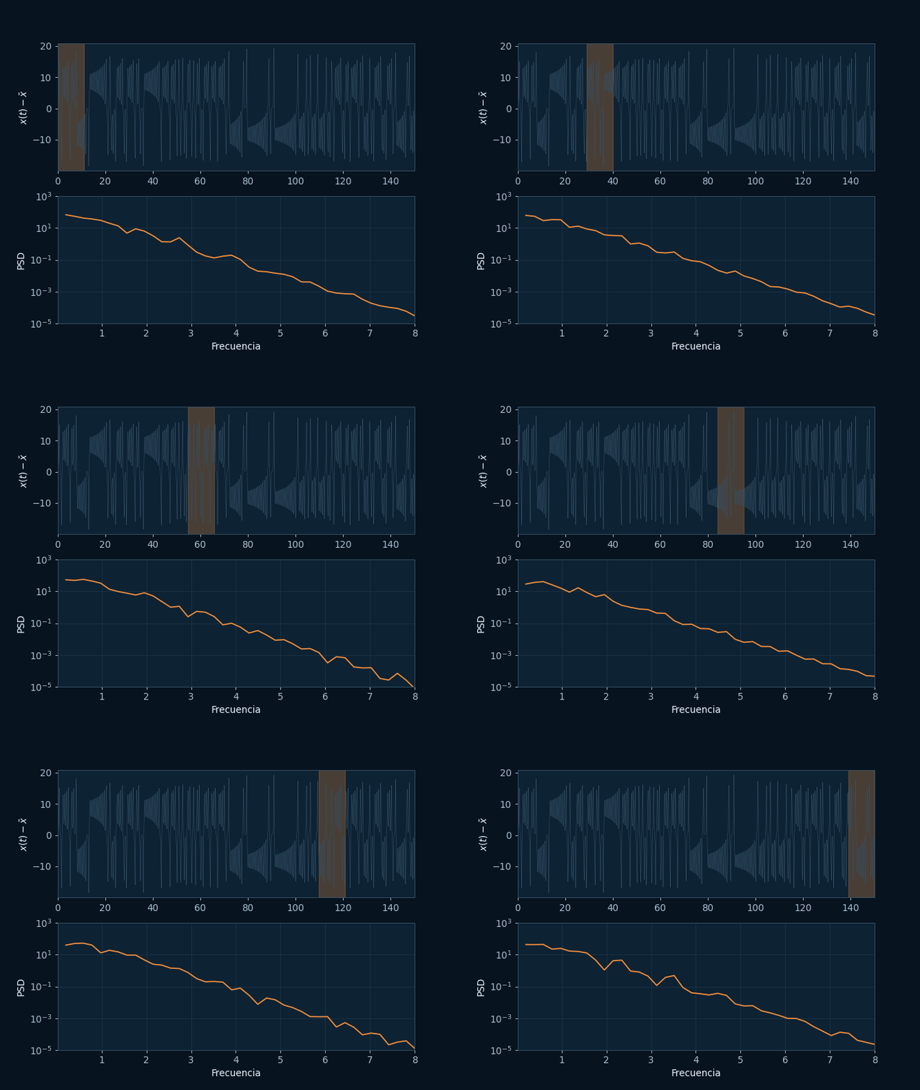
A simple periodic signal gives sharp peaks, whereas an irregular trajectory can spread power over broader bands. The animation changes the retained observation window to show why sampling step, transient removal, and window length must be reported.
Which frequencies appear in a time series?
Welch PSD and Spectral Reading
Definition: The Spectrum tab offers a Welch power spectral density and an amplitude spectrum. Both convert sampled time-domain data into frequency content, but they report different quantities.
Watch for: A spectrum supports classification when it is combined with trajectory, convergence, and sensitivity diagnostics.
The GIF loads only when requested.
The Sprott B example links a compact algebraic rule to a simulated orbit. The toolbox decodes the function, discards transients, chooses a projection, and applies high-contrast visual controls; the animation then reveals how the curve is traced in time.
How can compact codes generate candidate dynamics?
Sprott Codes and Generating Functions
Definition: A Sprott-style code is a compact recipe for a map or flow. The family symbol, dimension, order, and coefficient characters are decoded into a mathematical function: x(n+1)=F(x(n)) for maps or dx/dt=f(x) for flows.
Watch for: A visual candidate requires longer simulations, varied initial conditions, smaller steps for flows, and diagnostics such as Lyapunov exponents.
Questions addressed by each numerical view
A graph is easier to interpret when its question is explicit. This table separates the evidence supplied by basin maps, coexistence plots, FFT, trajectories, and convergence diagnostics.
Plot
Useful for answering
Additional evidence required
2D/3D trajectory
Where the orbit moves and whether it remains bounded.