Sprott Explorer

Decode compact Sprott-style codes into maps or flows, simulate them, apply local filters, search records, and render candidate dynamics.

Purpose Generate and inspect candidate dynamics

Evidence Level Visual triage and follow-up evidence

Question and result

Calculation performed

Decode, simulate, filter, visualize, and organize Sprott-style maps or flows as reproducible candidates for later numerical investigation.

GUI tab

Explorador Sprott

Configuration and calculation

Control sequence

Open a built-in example, generate a compact code, or load a user-owned local dictionary record.
Decode the family, dimension, order, coefficients, equations, and whether the definition is a map or a flow.
Use the fixed starting vector with every component equal to 0.1, then choose iterations or total time, transient, and an appropriate step and method for flows.
Simulate, retain bounded non-collapsed trajectories, and inspect several projections, point-density settings, and color modes.
Store promising simulations in the local gallery and export the numerical and explanatory artifacts needed to reproduce the view. Use Inventario local only to index reference files and send a selected .DIC to Ejemplos.

Record

Computed data

An explicit decoded map or flow together with a finite simulated trajectory and one or more candidate visualizations.
A local record that preserves the code, numerical settings, projection, and visual configuration used for the candidate.

Scientific reading

Interpretation criteria

A bounded structured rendering is a candidate for deeper analysis. Its evidence grows with transient, step, duration, projection, and re-simulation checks; alternative initial conditions require an external study.

The code, decoded equations, and simulation settings define the scientific object; point size, alpha, and color control its visual presentation.

Files

Experiment record

Export figures as PNG, PDF, or SVG; preserve metadata as JSON, trajectory values as CSV, and the generated explanation as Markdown when those artifacts are needed.
Record the code, family, decoded equations, dimension, map/flow type, fixed starting vector (0.1 in every component), method, step or iterations, duration, transient, divergence threshold, random seed, stopping criterion, maximum attempts, projection, and visual preset.

Applications

Questions addressed by the calculation

Teaching how compact codes become explicit maps, flows, trajectories, and projections.
Screening many generated definitions before allocating longer numerical studies.
Building a reproducible local gallery or dataset of candidate dynamics and their settings.

Scope

Evidence conditions

Visual triage can retain numerical artifacts, long transients, periodic orbits, or projection effects that resemble chaotic structure.
Passing the local filters identifies a candidate that requires chaos, attraction, robustness, and uniqueness diagnostics.
Hidden-attractor localization, classification, and certification require the dedicated HAFO mathematical engine and its validation workflow.

Current Toolbox Chaos Sprott Explorer interface — The current Sprott Explorer organizes nine workspaces: Inicio, Teoria, Codigos, Exploracion, Ejemplos, Tutorial, Galeria, Inventario local, and Backend explicado.

High-contrast Sprott B orbit with the title supplied in its caption — A public Sprott example rendered as a phase-space orbit. This caption provides its interpretation and keeps the plot reusable across contexts.

Hénon map showing stretching and folding at high contrast — Iterated-map projection: successive images make stretching and folding readable, with the title supplied in the surrounding guide.

Generated Sprott-style 4D map projected with fourth-coordinate color — 4D projection: the visible plane shows two coordinates while a fourth coordinate is encoded with color.

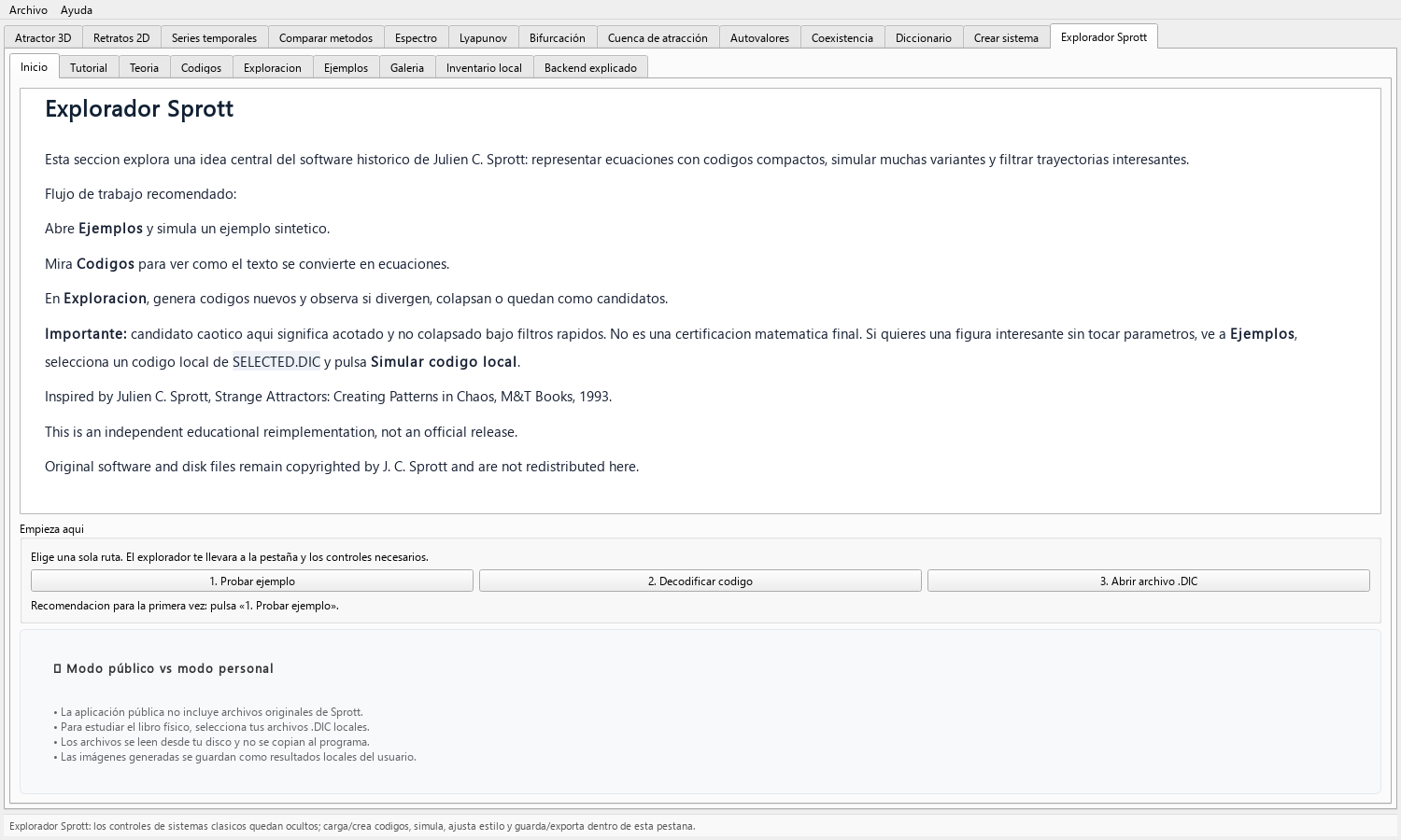
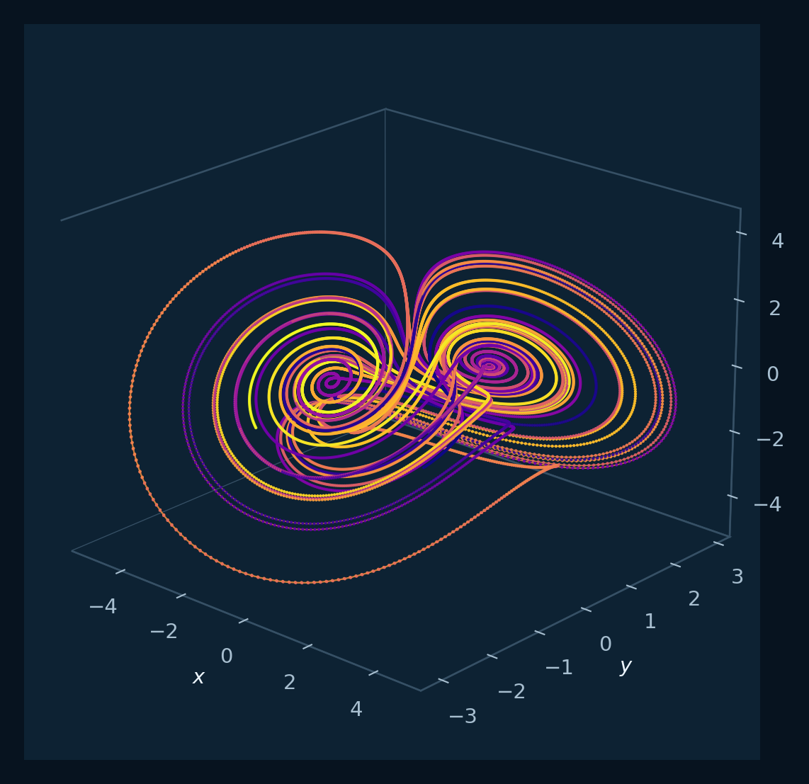
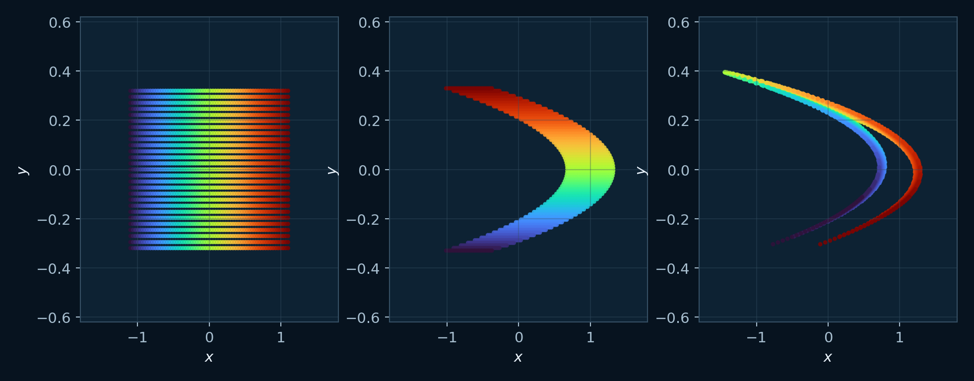
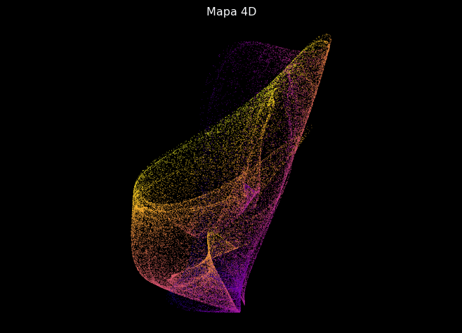
Sprott Explorer workflow

Open Sprott Explorer and choose Inicio → 1. Probar ejemplo, or open Ejemplos and select a recommended synthetic case.
Select Simular con estilo recomendado to load a coherent projection, palette, density, transient, and numerical scale.
Change one display or simulation control at a time and compare whether the geometric structure remains readable.
Export an image and, when the run will be analyzed elsewhere, the trajectory CSV and metadata JSON.
Save useful cases in the local gallery for re-simulation and comparison while retaining the source dictionaries intact.

Sprott Explorer workspaces

Codigos: decode, generate, and search compact records for maps and flows.
Exploracion: select projections, palettes, color variables, density, bands, point size, and transparency.
Ejemplos: run bundled synthetic maps and flows, including didactic fixed-point and divergence cases.
Diccionario: read a local .DIC resource in place while preserving the original file.
Galeria: preserve generated cases with their simulation and visual metadata, then reopen or re-simulate them.
Inventario local: index local reference files in place and send a selected .DIC to Ejemplos.
Export: save PNG, PDF, or SVG graphics, CSV trajectories, JSON metadata, galleries, and a Markdown explanation of the pipeline.

Rendering and clipboard controls

Control	What it changes	Invariant under the visual control
Fondo	Background color of the canvas and exported figure.	The decoded equations and simulated trajectory.
Modo dibujo	Representation as points, line, line plus points, or density view.	The numerical samples already produced by the simulation.
Max puntos	Visual subsampling after the transient so a dense render remains responsive and readable.	The stored or exported simulated data; it limits drawing only.
Bandas	Quantization of a continuous color scale into a declared number of bands; zero keeps continuous color.	Coordinates, iteration order, and dynamics.
DPI export	Raster resolution used for PNG and PDF-oriented exports.	Simulation accuracy or number of trajectory samples.
Mostrar ejes, Mostrar grid, Aspect ratio igual	Axes, reference grid, and geometric scaling of the view.	The underlying trajectory; equal aspect changes the displayed distance scale while preserving coordinate values.
Copiar codigo, Copiar cita	The compact code or supplied citation placed on the clipboard for a record or caption.	The current equations, numerical settings, and rendered result.

Sprott codes, equations, and update rules

A Sprott-style code is a compact recipe for a dynamical system. The code is decoded into algebraic terms, coefficients, dimension, and update type; the toolbox then simulates the resulting map or flow.

The educational value is that a short symbolic record can generate many different phase portraits. Students can see how simple deterministic functions produce fixed points, cycles, dense clouds, folded bands, or apparently chaotic attractors.

1. Family

The first symbol selects a family. In the toolbox grammar, families A-D are 1D maps, E-H are 2D maps, I-L are 3D maps, M-P are 4D maps, Q-T are 3D flows, and U-X are 4D flows.

2. Dimension and order

The family implies the number of variables and the polynomial terms that may appear. Maps are iterated directly; flows are integrated as differential equations.

3. Coefficients

The remaining characters encode coefficients. The decoder maps characters into numeric weights and attaches those weights to the monomials allowed by the selected family.

4. Function

The decoded record becomes an explicit function: x(n+1)=F(x(n)) for maps, or dx/dt=f(x) for flows. This function is what the toolbox actually simulates.

Candidate search workflow

The searcher is a triage workflow. It tries many compact recipes, simulates them with bounded numerical settings, rejects obvious failures, and retains visually structured candidates for deeper analysis.

Generate or load a compact code.
Decode the code into equations, dimension, order, coefficients, and update type.
Simulate the map or flow from the current fixed starting vector, with every component equal to 0.1.
Discard transient points so the figure represents the established trajectory.
Reject obvious failures such as divergence, collapse, NaN values, or empty ranges.
Render several projections and color modes to see whether the structure survives visual changes.
Promote promising candidates to longer simulations and independent diagnostics.

Presets, Criteria, and Re-simulable Attempts

A simulation preset changes a coherent group of controls at once: map or flow type, dimension, polynomial order, iterations, discarded transient, integration step, and flow method. Start with a recommended map or short RK4 flow preset, read the applied values shown below the selector, and then change one control at a time. Visual presets are separate: options such as Color por profundidad, Alta densidad, and Didactico change projection and rendering while retaining the decoded equations.

Set Semilla aleatoria before Generar codigo or Buscar candidato. Reusing the seed with the same family, dimension, order, and search controls reproduces the generated code sequence; when local .DIC entries participate, also record the filter and selected starting row.
Set Intentos maximos to bound how many codes Buscar candidato may test in one run. A larger value explores more candidates but also increases computation time.
Choose the minimum stopping criterion: candidate_chaotic for the quick candidate filter, acotado for a bounded result, or cualquier no divergente for the widest acceptance rule available.
Read the attempts table alongside the final image. Each row reports attempt number, code, state, reason, x/y ranges, and a quick Lyapunov indicator.
Double-click any row to load that code back into Exploracion and simulate it again under the currently declared numerical and visual settings.

The stopping criterion controls triage. In particular, candidate_chaotic and the quick Lyapunov column identify records for longer simulations and independent diagnostics, including a convergence-aware Lyapunov analysis.

Local .DIC Workflow

The Ejemplos workspace reads user-provided .DIC files from disk. Select an automatically detected SELECTED.DIC, BOOKFIGS.DIC, or SPECIAL.DIC, or choose a file manually. The application reads the source in place and preserves the dictionary outside the project.

Choose a load limit of 350, 500, 1000, or Todos. Use a smaller limit for a quick inspection and the complete option only when the full table is needed.
Filter the loaded table by simulation support, map or flow type, dimension, family, parser outcome, or the displayed F and L criteria. The status line reports how many recognized entries remain visible.
Select a row to inspect its source line, code, family, dimension, order, metrics, support state, and decoded details. Double-click it, use Simular codigo local seleccionado, or apply Simular con estilo recomendado.
For a local batch, choose N = 10, 25, or 50 and press Generar galeria local desde este .DIC. Only the first N currently visible records are simulated, so apply the intended filter before starting.

Gallery and Local Inventory

Guardar en galería stores a locally generated render, thumbnail, decoded code, simulation configuration, visual style, and source identity. In Galeria, select an entry to inspect those values, open the render, re-simulate the code, restore its style for editing, or export the displayed PNG. Re-simulation restores the saved iterations, transient, step, method, divergence threshold, and visual configuration before running the code again.

Inventario local serves a different purpose. Select a folder to list recognized local references by name, path, type, size, and category; optionally calculate a SHA-256 hash when file identity matters. The inventory lists files in place and preserves their contents. A selected .DIC can be sent to Ejemplos for the read-only loading and simulation workflow described above.

Book Reading Mode

After loading a local BOOKFIGS.DIC or another compatible dictionary, enable Modo lectura del libro. The view reuses the entries already in memory and lets you restrict the table to a line interval that corresponds to the part of the physical reference you are consulting.

Select a row to inspect the code, family, dimension, order, F/L values, support information, and decoded detail. Double-click to simulate it, use the recommended-style button for a family-appropriate rendering, send it to Codigos for detailed decoding, save a generated image to the local gallery, or copy the supplied academic citation. The original .DIC remains unchanged.

Backend Explained and Markdown Export

Backend explicado converts the code currently shown in Exploracion into a didactic account of the complete GUI pipeline: input cleaning, family decoding, monomial count, coefficient matrix, explicit equations, the fixed starting vector, simulation method, classification criteria, and visual configuration. It can explain the text of a code before a run; after a simulation, it also incorporates the active rendering settings.

Place the target code in the Exploracion code field and verify iterations, transient, step, method, and current visual preset.
Press Explicar código actual and compare the displayed equations and simulation contract with the generated figure.
Press Exportar explicación Markdown to save the same structured explanation as a portable .md file for a laboratory record or teaching handout.

The explanation documents the interface workflow for the code. Proof of chaos or hiddenness requires the dedicated mathematical evidence.

Code decoding and trajectory rendering

Decode: split the compact code into family, dimension, polynomial order, and coefficient list.
Build the function: combine coefficients with allowed monomials to form F(x) for maps or f(x) for flows.
Simulate: iterate maps directly or integrate flows with Euler/RK4 using a chosen step size.
Discard transient: remove the initial segment so the figure reflects established long-term behavior.
Project: choose x-y, x-z, y-z, 3D, or a 4D projection where the hidden coordinate appears as color.
Filter: reject trajectories that diverge, collapse to a point, leave the plotting range, or show obvious numerical failure.

Simulation and rendering controls

Iterations or total time

Too few points can miss the attractor. Too many points can overplot into a solid mass unless point size and alpha are reduced.

Transient length

A startup spiral or jump can look interesting but disappear after enough transient points are removed.

Step size for flows

Euler or RK4 step size changes numerical stability. A large step can create false bounded shapes or divergence.

Fixed starting vector

The current Explorer simulation fixes every starting component at 0.1. Interpret each candidate under that declared start.

Projection

2D, 3D, and 4D color projections reveal different aspects of the same data. A fourth coordinate can be encoded by color.

Alpha and point size

Dense maps need smaller points and lower alpha so returns remain visible instead of forming an opaque block.

Candidate screening and follow-up analysis

A candidate image is a hypothesis. If it is bounded, non-collapsed, and visually structured, it deserves further inspection. The next steps available in the GUI are to run longer simulations, reduce the integration step for flows, compare projections, estimate Lyapunov exponents in the appropriate dedicated workflow, and check whether the apparent structure survives. The Explorer itself keeps every starting component fixed at 0.1.

This is why the toolbox labels quick results conservatively. A visual candidate can guide exploration, but chaos claims require numerical diagnostics and reproducibility.

Evidence conditions for candidate dynamics

Calling every dense cloud chaotic: numerical noise, bad projection, or too many overplotted points can mimic complexity.
Skipping transients: a startup spiral can look interesting but disappear after enough iterations.
Establishing initial-condition robustness: Sprott Explorer uses the fixed vector with every component equal to 0.1; an external study with alternative initial conditions supplies this evidence.
Interpreting candidate_chaotic: this quick filter outcome guides longer simulations and formal mathematical classification.

Scope Boundary: Toolbox Chaos and Hidden Attractors FO

Sprott Explorer is a GUI for generating, simulating, filtering, visualizing, and organizing candidate dynamics. The Hidden Attractors FO engine provides the separate, documented mathematical workflow for hidden-attractor localization and classification.