Toolbox Chaos procedure
Time Series
Read each state variable against time or iteration, identify transients and numerical warning signs, and prepare signals for spectral or comparative analysis.
Question and result
Calculation performed
Establish what the computed state does over the observation window before interpreting a phase portrait or diagnostic.
Required configuration
- Choose a model and numerical contract, or retain a compatible shared trajectory from another tab.
- For maps, the horizontal axis records iteration number. Continuous-time models use physical time.
Panel and figure
Displayed quantities
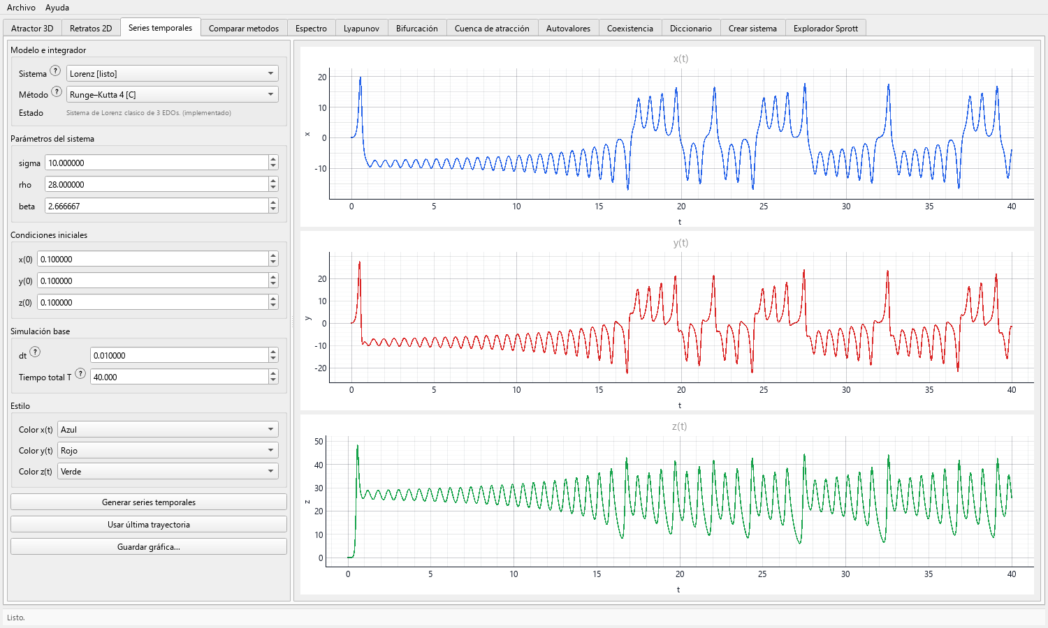
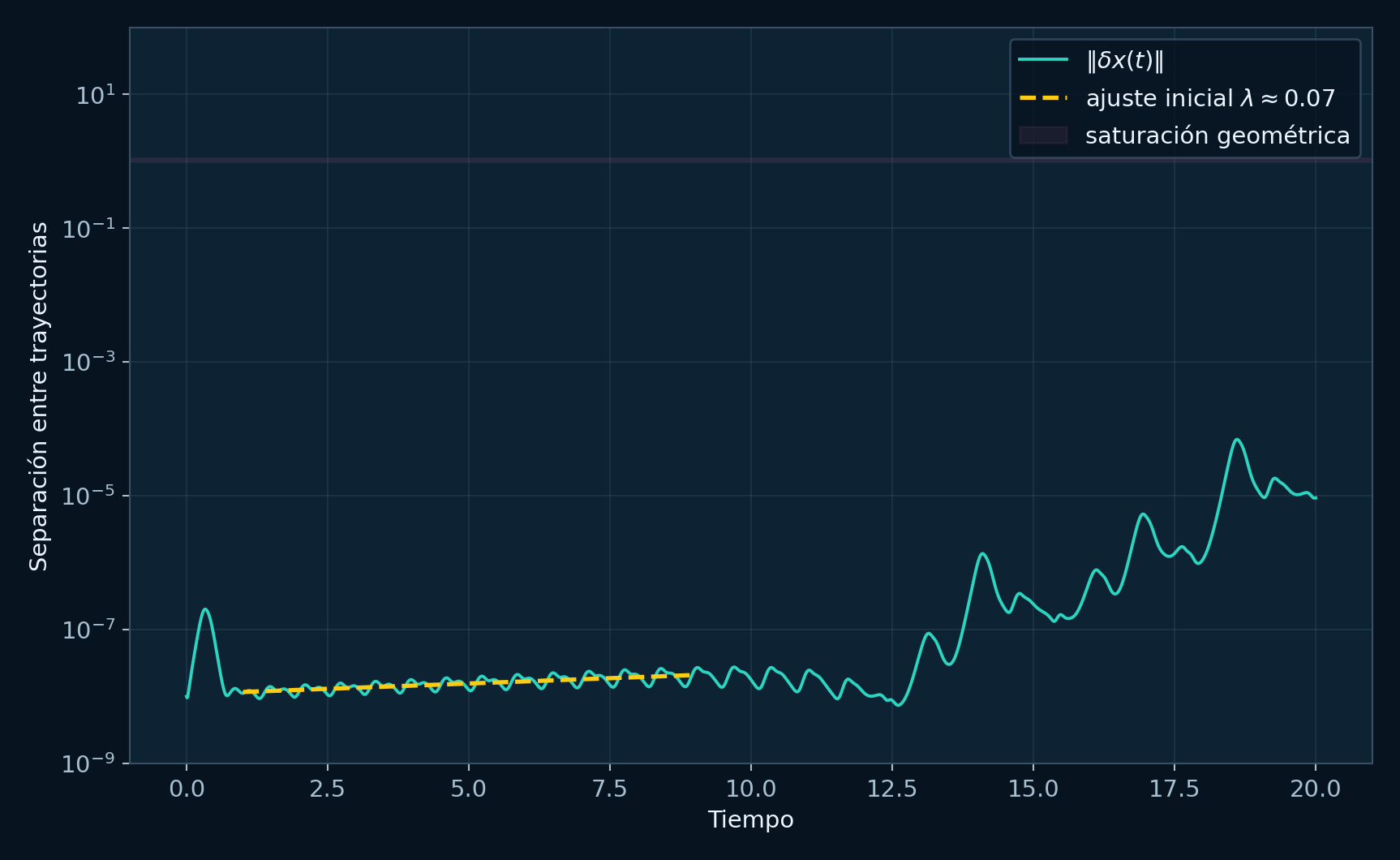
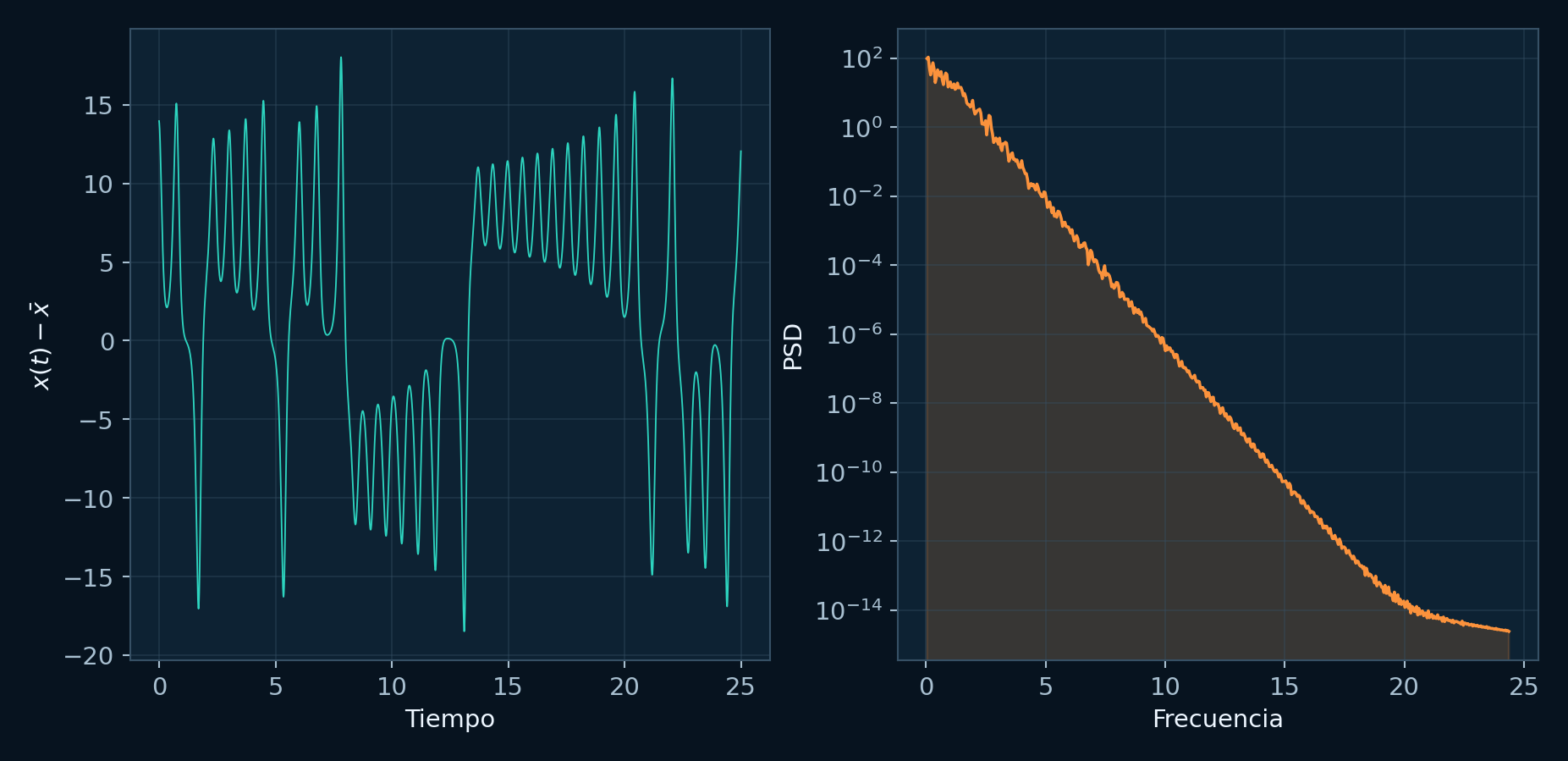
Configuration and calculation
Control sequence
-
Generate or reuse the trajectory
Select the system and either press Generar series temporales or use the last trajectory created for the same model.
When comparing views, reuse is preferable because it eliminates an unintended difference in integration settings.
-
Inspect the beginning of the record
Identify rapid approach, overshoot, or drift that belongs to the initial transient. Record the transient policy and the retained time interval before cropping a trace.
A signal with unbounded growth or an invalid state calls for a review of step size, parameters, and initial state before interpretation.
-
Compare variables
Use separate state panels and colors to examine phase shifts, relative amplitude, slow envelopes, bursts, plateaus, or switching events.
Avoid comparing raw amplitudes across variables with different physical units unless a documented normalization is applied outside the GUI.
-
Check observation length
Extend the duration to determine whether an apparent steady regime persists. A short nearly periodic segment can be a transient or a window inside a longer irregular record.
For slow–fast models such as Hindmarsh–Rose, ensure the horizon covers both several slow cycles and fast spikes.
-
Perform a resolution check
Repeat with a smaller step for flows. Compare waveform scale, event timing over early intervals, and qualitative regime.
Late pointwise divergence is expected in sensitive regimes; use convergence of statistics or qualitative features instead of demanding identical long traces.
-
Export and hand off
Save the time-series grid. If continuing to Espectro, use the same trajectory and declare the transient removed there.
Include the horizontal-axis meaning, units if known, sampling step, and total window in captions or experiment notes.
Record
Computed data
- One aligned signal per displayed state variable over a known time or iteration window.
- A documented transient interval and a judgment about whether the remaining window is long enough for the intended analysis.
Scientific reading
Interpretation criteria
Periodic repetition, quasiperiodic modulation, intermittent bursts, and irregular fluctuations can often be distinguished provisionally in time, but each pattern requires corroboration.
An irregular signal may result from deterministic chaos, a transient, insufficient resolution, delay-model history effects, or numerical instability. Use the corresponding diagnostics to distinguish these possibilities.
Files
Experiment record
- Record step or iteration index, duration, and transient handling.
- Preserve variable names, units, and any color convention.
- Use the same window when comparing parameters or methods.
Applications
Questions addressed by the calculation
- Detecting transients before spectral or Lyapunov analysis.
- Studying oscillations, slow–fast bursting, switching, and map iterations.
- Communicating temporal behavior that is hidden by a phase-space projection.
Scope
Evidence conditions
- A chaos claim combines time-series observations with resolution checks and suitable diagnostics.
- Aliasing and inadequate sampling can alter apparent oscillations and any downstream spectrum.
- Basins, attraction, and hiddenness require workflows that sample initial conditions and apply the relevant criteria.