Toolbox Chaos procedure
2D Phase Portraits
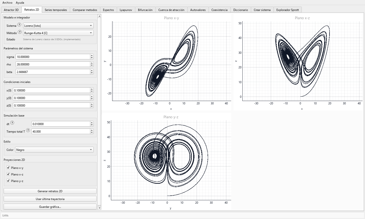
Inspect selected pairs of state variables, compare projections from the same run, and avoid confusing a flattened view with the full state space.
Question and result
Calculation performed
Use pairwise projections to reveal relationships, folds, loops, and return geometry while preserving the identity of the source trajectory.
Required configuration
- Have either a compatible last trajectory or a complete local simulation setup.
- Know which state labels correspond to each plotted axis.
Panel and figure
Displayed quantities
Configuration and calculation
Control sequence
-
Select the system and source
Choose the same system as the shared trajectory and press Usar última trayectoria, or enter a fresh numerical contract and run locally.
When the interface reports a system mismatch, simulate the selected system locally or return to the correct model.
-
Choose variable pairs
Enable the available pairwise planes. For three displayed states these are normally x–y, x–z, and y–z; higher displayed dimensions can provide more combinations.
Keep at least two projections when diagnosing whether an apparent crossing or loop is a flattening artifact.
-
Set a consistent visual style
Choose a color with enough contrast and retain equal aspect where provided to support geometrically consistent comparison.
Use the same style for a controlled series unless color itself encodes a declared experimental condition.
-
Read projection-specific structure
Look for repeated loops, folded bands, symmetry, narrow channels, clusters, and regions visited only during the transient.
Compare every observation with another projection or with the time series before assigning a dynamical meaning.
-
Repeat under a controlled change
Vary one parameter, initial-state component, step, or duration. Keep the remaining contract fixed and name the changed quantity in the export.
For parameter intervals, use the bifurcation workflow and retain the sampled parameter values.
-
Export the grid
Use Guardar gráfica... to save the complete selected projection grid. Confirm that axis labels remain readable at the intended publication size.
If individual panels are needed, keep the complete grid as the provenance record and state how any crop was produced.
Record
Computed data
- A grid of selected pairwise portraits generated from one known trajectory.
- A list of features that are consistent across projections and features that appear only after flattening.
Scientific reading
Interpretation criteria
A projected crossing can represent states separated in an omitted coordinate. A closed-looking loop may also conceal slow drift outside the plane.
Pairwise portraits are strong descriptive tools. Full invariant-dynamics classification requires diagnostics that cover the modeled state dependence.
Files
Experiment record
- Name every variable pair and state whether the trajectory was reused.
- Record the full simulation contract even though the panel shows only geometry.
- Keep aspect-ratio and crop choices consistent across comparisons.
Applications
Questions addressed by the calculation
- Visual comparison of coupled variables.
- Preparation of figures for lectures, posters, and exploratory reports.
- Selecting a useful observable pair before a basin, section, or return-map study.
Scope
Evidence conditions
- Projection overlap can correspond to states separated along an omitted coordinate.
- Sensitivity, spectral content, and local stability are evaluated with their corresponding diagnostics.
- The panel visualizes selected trajectories; hidden-attractor localization belongs to Hidden Attractors FO.