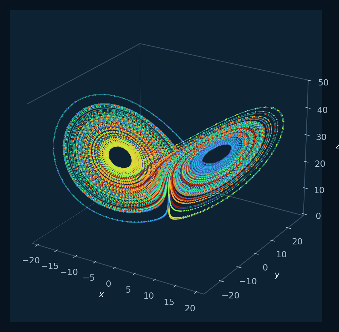
Lorenz trajectory at the standard parameter set

Set up parameters, run your first simulation, and compare 3D phase space with projected 2D phase portraits for the Lorenz system.

Difficulty Level Beginner

Question What does a trajectory look like?

Question and result

Calculation performed

Run a reproducible classical Lorenz simulation and connect its 3D geometry with two-dimensional projections and coordinate time series.

GUI tab

Atractor 3D, followed by Retratos 2D and Series temporales

Configuration and calculation

Control sequence

Select Lorenz and retain the classical parameter values sigma=10, rho=28, beta=8/3 with initial state (1,1,1).
Choose RK4, dt=0.01, and a duration long enough to move beyond the visible startup segment.
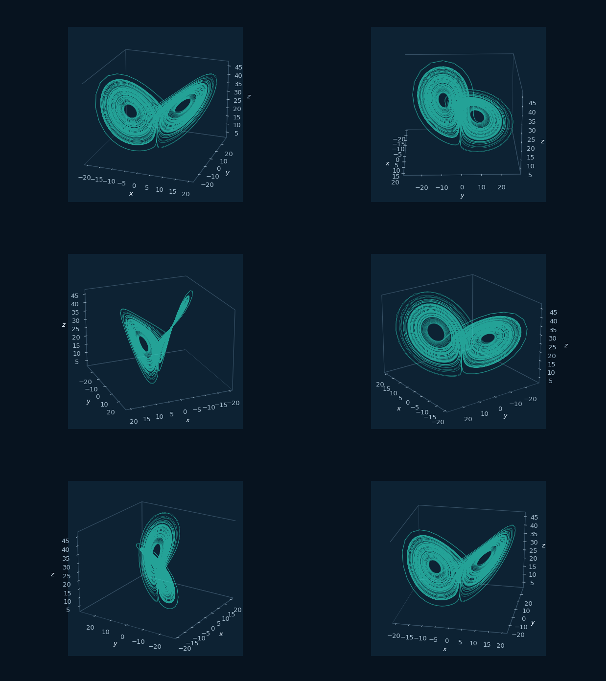
Generate the 3D trajectory and rotate it to inspect both lobes and the folded geometry.
Open Retratos 2D and Series temporales with the same simulation inputs, or reuse the compatible last trajectory when that option is available.
Repeat with a smaller step or longer time before using the output in a research record.

Record

Computed data

A bounded butterfly-shaped 3D trajectory with repeated visits to both Lorenz lobes.
Consistent x-y, x-z, and y-z projections plus time traces derived from the same numerical setup.

Scientific reading

Interpretation criteria

The curve is a path through state space; the lobes and switching describe the computed evolution of x, y, and z.

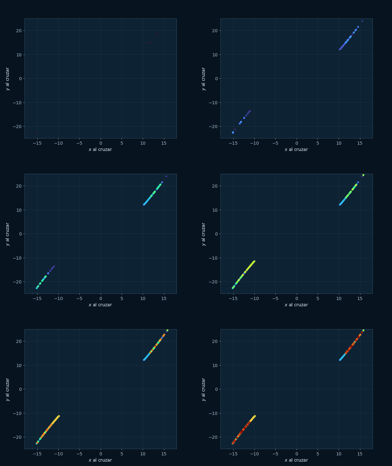
The projections reveal different folds, while the time series reveal switching order. Inspect the three-dimensional view to recover geometric depth.

Files

Experiment record

Save each required figure only after labels, line density, color, and projection are legible.
Record the system, ordered parameters, initial state, method, dt, duration, transient treatment, plotted coordinates, and whether a prior compatible trajectory was reused.

Applications

Questions addressed by the calculation

Introducing phase space, deterministic sensitivity, transients, and projection effects.
Checking numerical settings before method comparison, spectral analysis, or Lyapunov estimation.
Producing reproducible reference figures for dynamical-systems teaching and research protocols.

Scope

Evidence conditions

One finite trajectory documents its declared initial condition and time horizon. Basin characterization requires a sampled region of initial conditions.
A familiar butterfly shape can be distorted or created by unsuitable step size, duration, or transient handling.
The visualization supplies geometric evidence. Establish chaos, global attraction, uniqueness, or hiddenness with the diagnostics and analyses appropriate to each claim.

Three-dimensional Lorenz trajectory with both lobes visible — Expected geometry: the trajectory winds repeatedly around one lobe, crosses the central region, and continues around the other. Color encodes time progression and leaves the three state variables on the axes.

Rotating view of the Lorenz attractor with the trajectory unobstructed by an embedded title — The rotation reveals the depth of the butterfly shape: both lobes occupy three dimensions and the transitions pass through a three-dimensional neck.

Lorenz trajectory accumulating oriented crossings on a Poincare section — Analysis reduction: retaining crossings with a declared orientation turns the continuous flow into a sequence of returns. The resulting point cloud summarizes recurrence, while the trajectory view retains the full path.

Lorenz simulation procedure

Open the 3D attractor workflow in the toolbox.
Choose Lorenz from the system selector.
Keep the classical preset values sigma = 10, rho = 28, beta = 8/3, and initial state (1, 1, 1).
Use dt = 0.01, total time around 40, and Runge–Kutta 4.
Run the simulation, then rotate the 3D canvas to check that both Lorenz lobes are visible.
Switch to 2D phase portraits and time series to compare projections and coordinate traces before exporting.

Lorenz equations and phase-space geometry

The Lorenz system is a system of three ordinary differential equations first studied by Edward Lorenz in 1963 as a simplified model for atmospheric convection. In the classical chaotic parameter regime, the trajectory traces a butterfly-like shape in three-dimensional phase space.

The axes are the state variables x, y and z. The curve records the history of the system state in phase space. The two lobes show that the orbit repeatedly visits two regions, while the switching time remains irregular.

Read the 3D plot together with the time series and the 2D projections. The 3D plot shows geometry, x(t), y(t), and z(t) show temporal evolution, and the 2D portraits reveal how pairs of variables fold and return.

Parameters, initial state, and integration horizon

rho: changing rho can move Lorenz from stable equilibria into lobe switching and chaotic motion.
Initial condition: nearby starts can follow similar paths briefly and then separate in the chaotic regime.
Step size: too large a dt can cause numerical divergence or a false-looking trajectory.
Total time: too short shows mostly transient; longer windows reveal the attractor geometry.
Projection: x-y, x-z, and y-z projections emphasize different folds; inspect the set of views together.