toolbox_chaos
v0.1.0
Python 3.10+ · PyQt6 GUI · v0.1.0 Stable

Toolbox Chaos: Graphical Simulation and Analysis of Dynamical Systems

The application configures models, integrates trajectories, generates diagnostics, and records the data required to repeat each numerical experiment.

Download Documentation GitHub Cite

About

Software version, DOI, platforms, and architecture.

Version
0.1.0
License
MIT License
Archive
OSF DOI 10.17605/OSF.IO/GQMJR
Platforms
Windows, macOS, Linux
Interface
13 scientific tabs and 38 registered systems
Built with
Python 3.10+, PyQt6, NumPy, Matplotlib
Architecture
Toolbox Chaos GUI + Hidden Attractors FO mathematical engine
Author
Maria Fernanda Moreno Lopez (Fer Moreno) / Xerkkun
Repository
github.com/Xerkkun/Toolbox-chaos

Simulation and Analysis Functions

Desktop tools for simulation, visual analysis, and reproducible figure generation.

3D
38 Registered Systems
Load flows, maps, delay models, neuronal systems, the Sprott A-S family, Lorenz-96, and a 4D hyperchaotic model from one selector.
2D
3D and 2D Geometry
Generate 3D trajectories, compare the xy, xz, and yz projections, and reuse the same simulation across views.
TS
Reusable Time Series
Inspect state variables over time and send the last trajectory directly to portraits or spectral analysis for immediate reuse.
RK
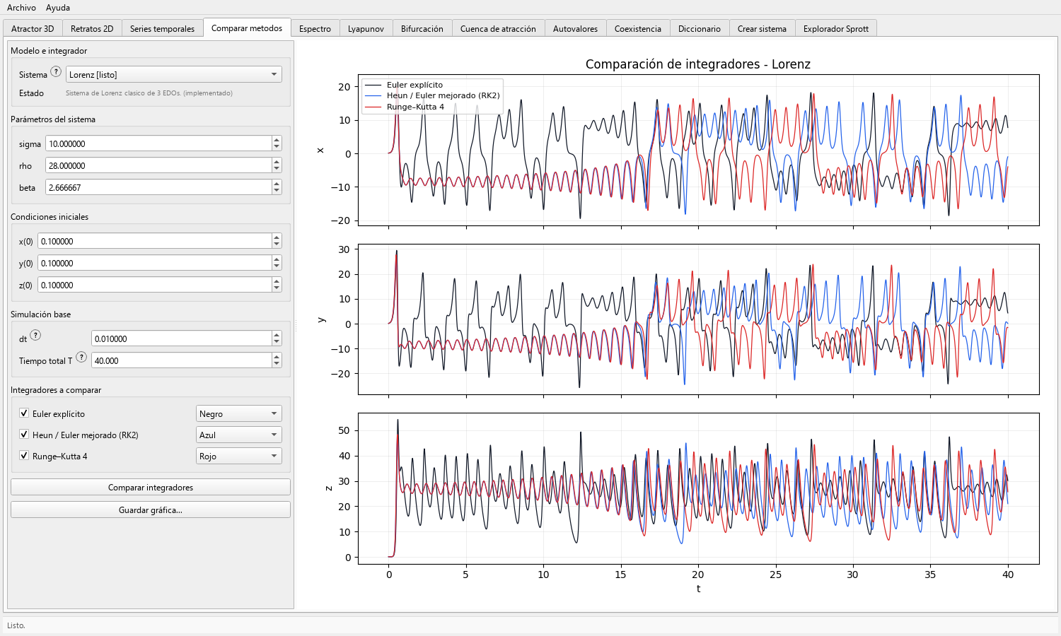
Integrator Comparison
Overlay Euler, Heun/RK2, and RK4 trajectories to study step-size sensitivity and select an appropriate numerical method.
PS
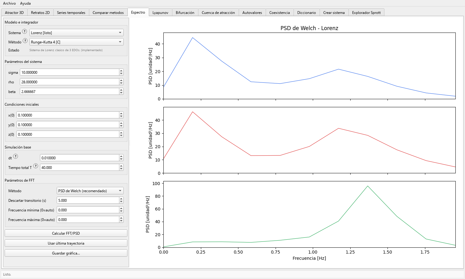
Welch PSD and Amplitude
Estimate a Welch power spectral density or amplitude spectrum with physical frequency units and a configurable transient.
EV
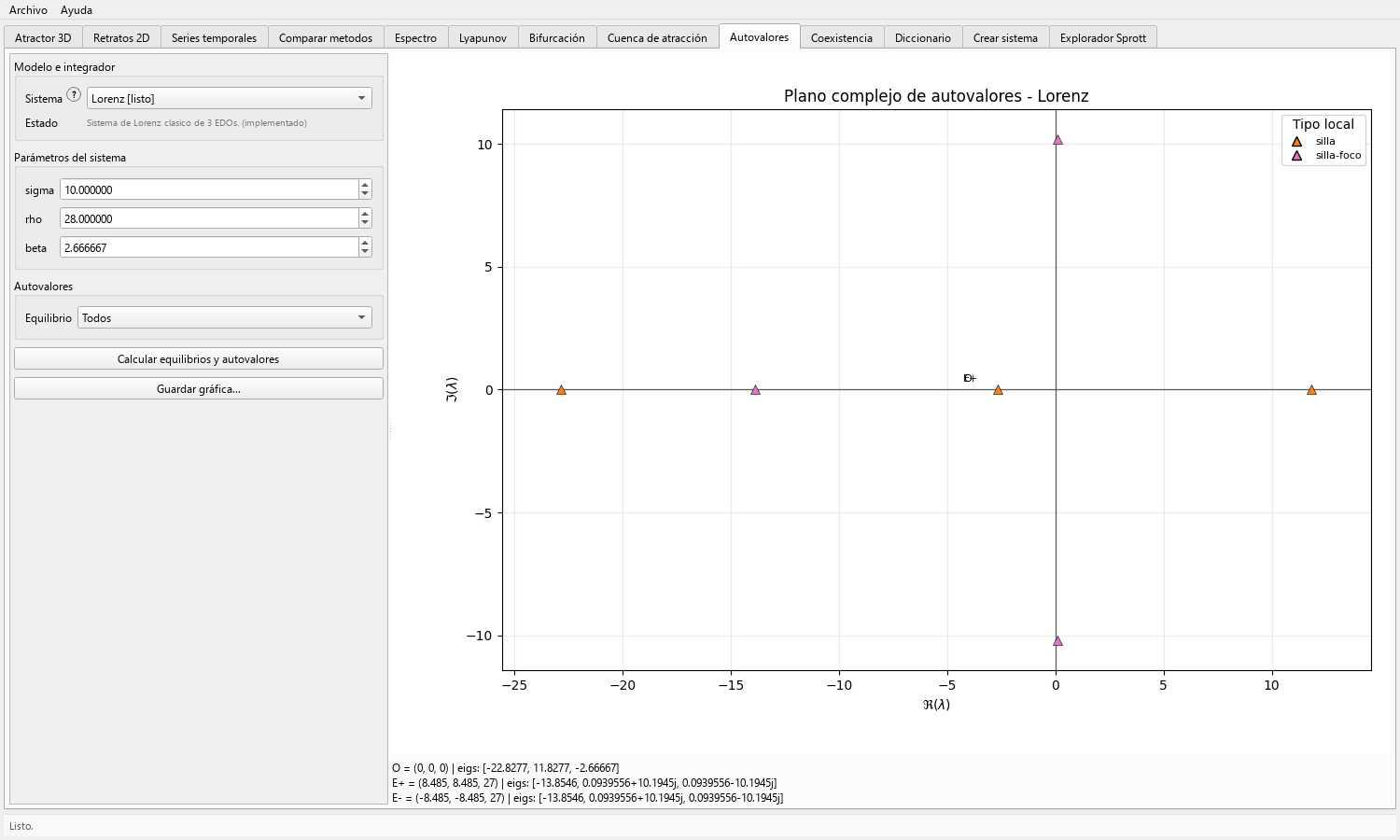
Equilibria and Eigenvalues
Locate equilibria of ODE flows, inspect eigenvalues in the complex plane, and read their local stability classification.
SP
Sprott Explorer
Decode and generate compact systems, run examples, search candidates, manage a local gallery, and export figures, trajectories, and metadata.
CO
Coexisting Attractors
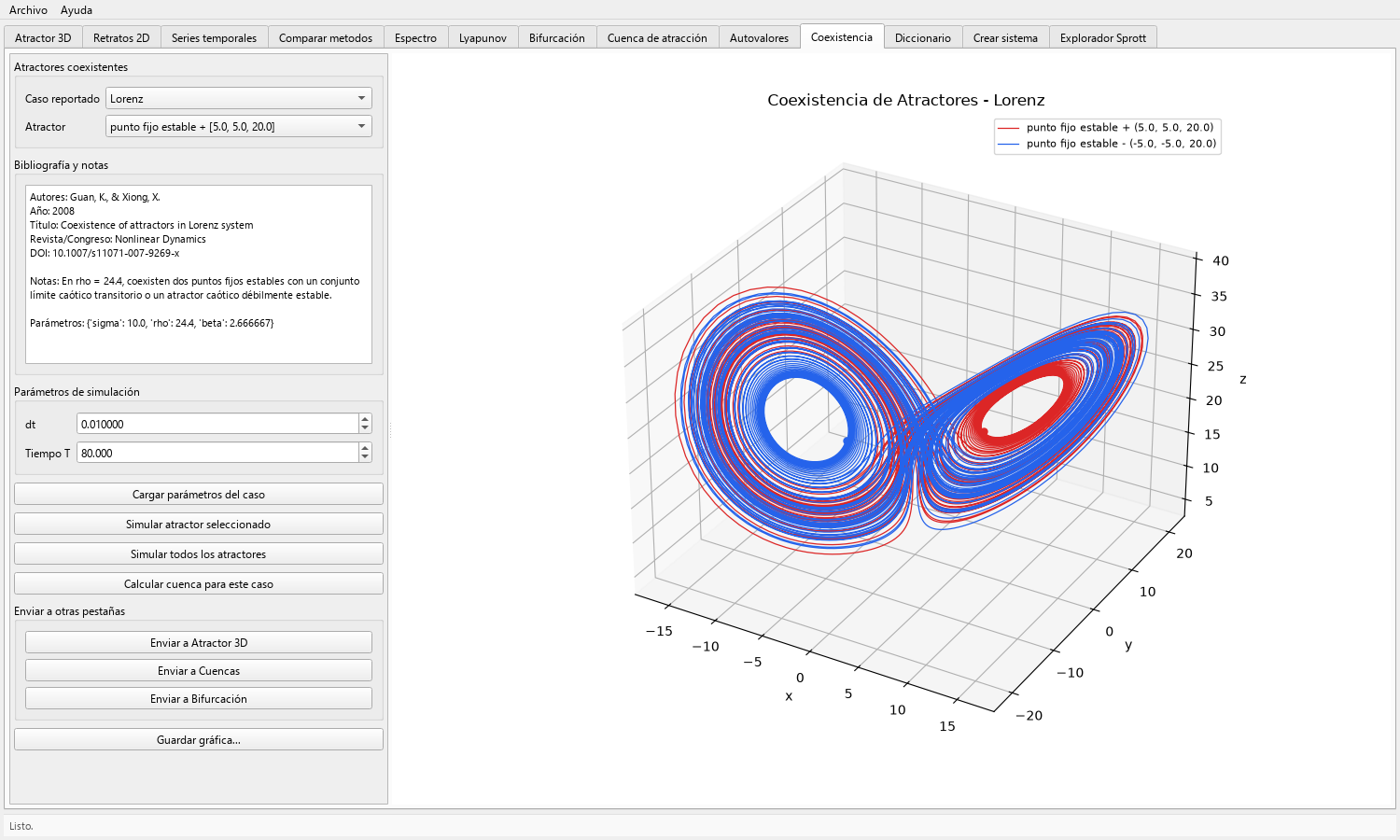
Compare multiple trajectories produced by one parameter set and different initial conditions in included reference cases.
BA
Basins of Attraction
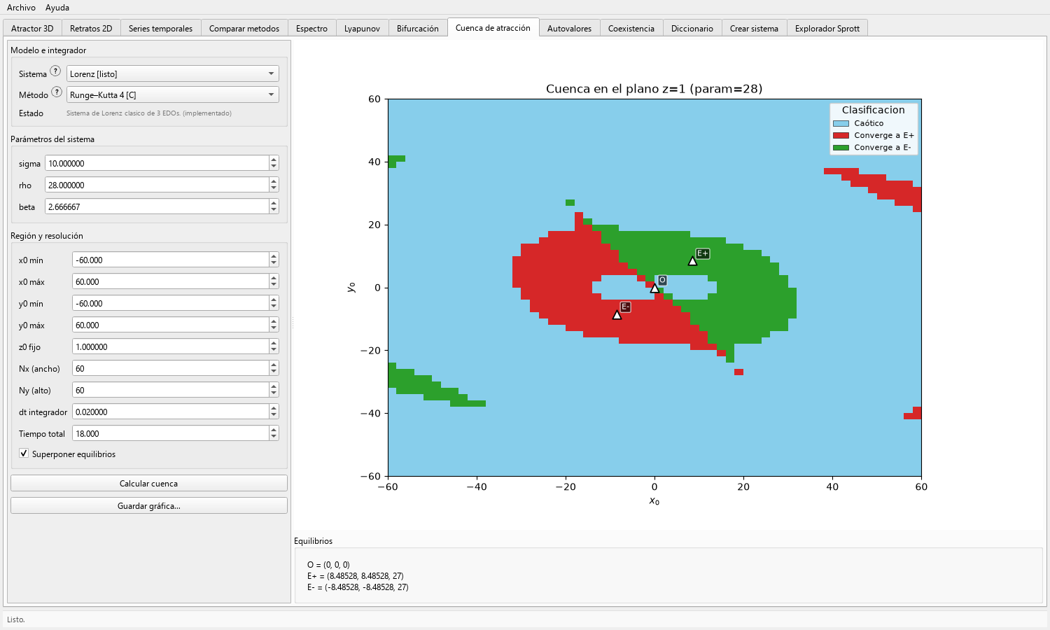
Classify a plane of initial conditions by the destination observed over the simulated horizon and inspect representative trajectories and equilibrium markers.
BF
Bifurcation Diagrams
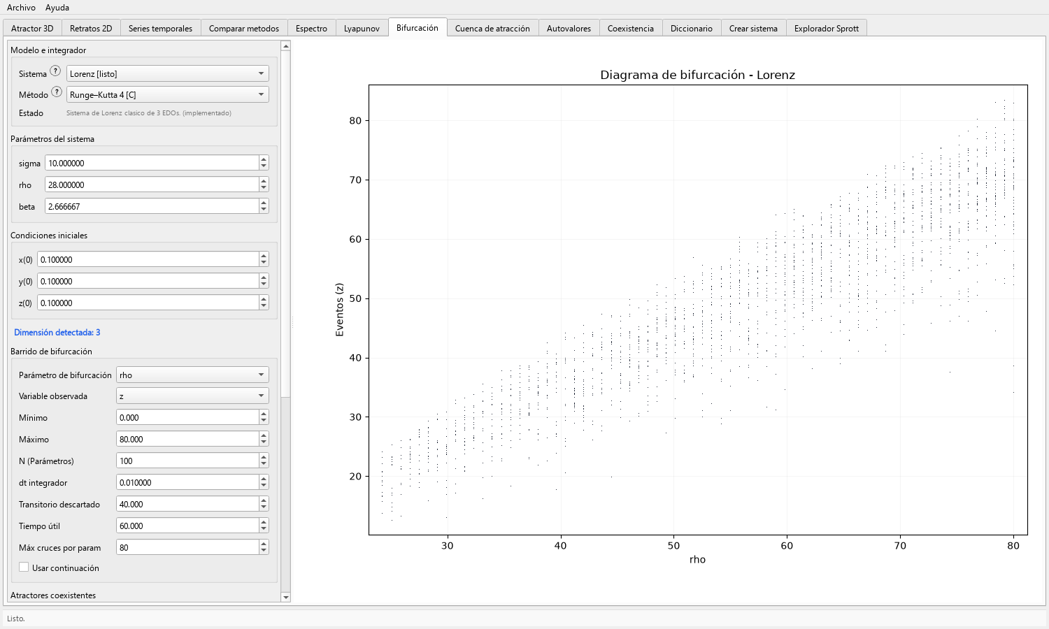
Sweep one parameter, discard the transient, retain an observable, and compare branches or attractor responses.
LY
Lyapunov Diagnostics
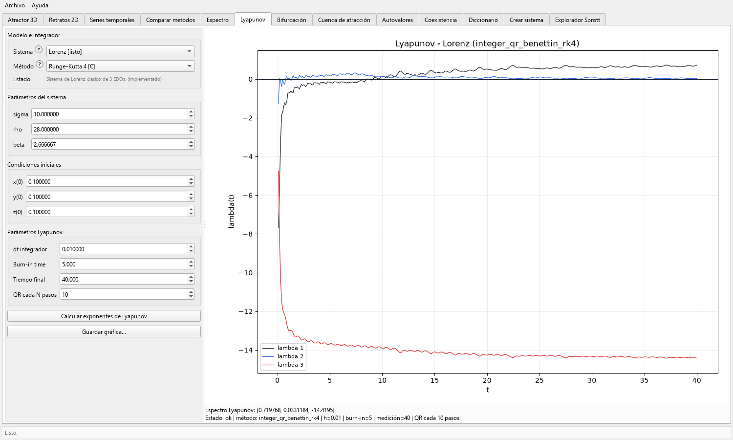
Estimate finite-time Lyapunov spectra for 3D ODE flows and inspect convergence before interpreting the result.
PDF
Local Scientific Dictionary
Open the bundled dictionary and supporting documents directly from the application while interpreting each diagnostic.
EX
Figure and Result Files
Save scientific figures and, in Sprott workflows, export trajectory CSV, metadata JSON, local galleries, and Markdown explanations.

Definitions linked to numerical results

Reading Trajectories and Diagnostics

The PDF dictionary and web guides connect dynamical-systems concepts with figures produced under explicit numerical contracts. This page identifies the available calculations, while each guide develops the configuration, result interpretation, and supporting data.

Study the dynamical-systems concepts -> Follow the complete university pathway in Learning →

Definitions and Reproducible Figures

The dictionary and web guides connect each definition with a reproducible figure and explain the quantity calculated by each diagnostic.

Basins, Bifurcations, and Lyapunov Rates

A basin map classifies initial conditions; the coexistence view contrasts destinations; a bifurcation diagram scans a parameter; and a Lyapunov plot estimates separation rates.

Parameters and Initial Conditions

Each example records the system, parameters, initial condition, projection, and retained window so another run can reconstruct the plot.

Compact-system exploration workflow

Sprott Explorer

The Sprott Explorer decodes compact descriptions inspired by J. C. Sprott's work on strange attractors. Starting from a generated example, it lets the user adjust the projection and graphical parameters to compute maps, flows, and dense phase-space representations.

The public examples record their computational settings. The guide develops the decoding logic, search filters, plotting choices, and the effect of each parameter.

Open the Sprott guide ->
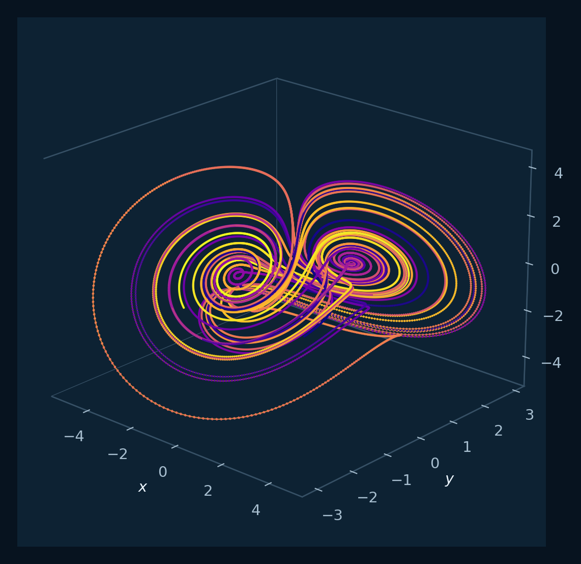
High-contrast continuous Sprott B flow
Sprott flow: geometry, projection, and integration method recorded in the caption
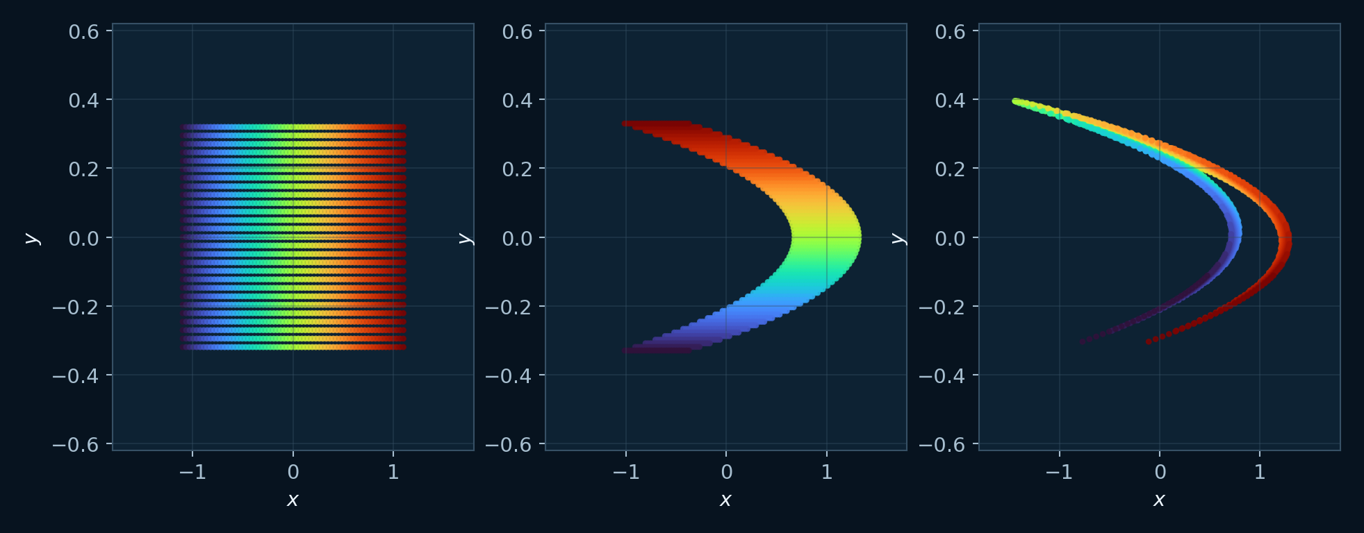
Hénon map showing stretching and folding
Iterated map: stretching, folding, and projection
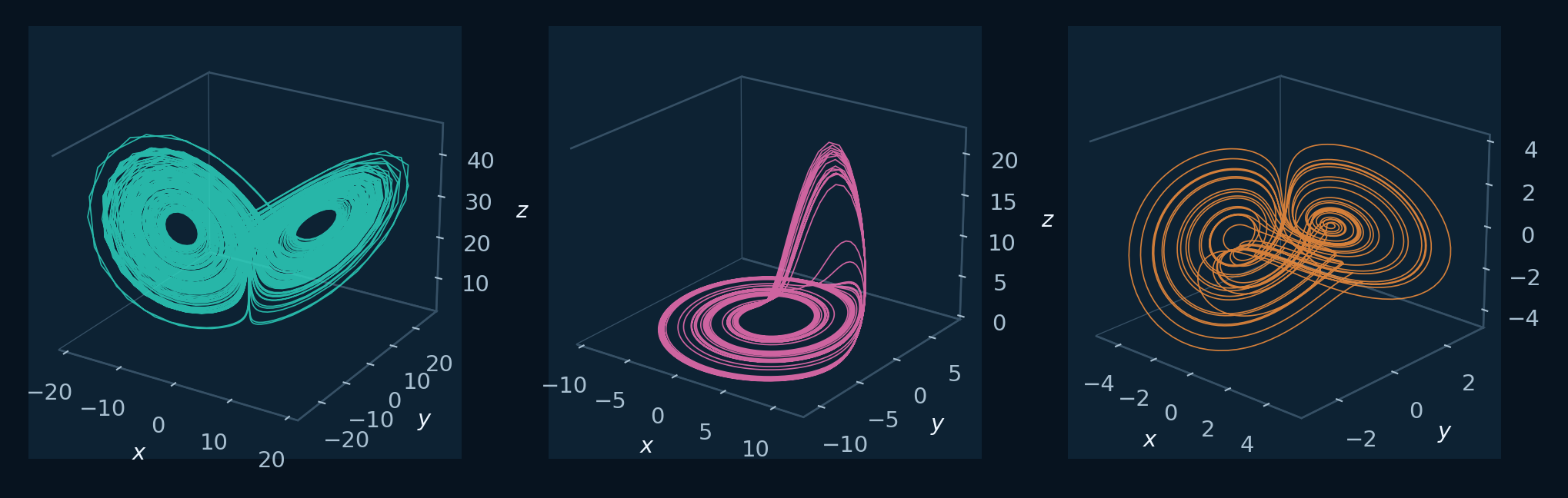
Coordinated comparison of Lorenz, Rössler, and Sprott geometries
Coordinated projections of Lorenz, Rössler, and Sprott

Numerical Experiment Sequence

The question determines the model, integration contract, refinement study, and files that document the run.

1

Choose a scientific question

Start from the view or comparison you need: trajectory geometry, time evolution, integration method, spectrum, bifurcation, basin, coexistence, or local stability.

2

Load a coherent preset

Use a registered system so equations, parameters, initial state, and integration scale begin in a known range.

3

Compute a low-resolution reference

Use a preliminary grid, a short sweep, or a small point set to verify the interval and estimate the computational cost.

4

Refine one control

Change one value at a time: time step, total time, transient, parameter range, projection, or density.

5

Relate trajectories, spectra, and stability

Connect geometry and time series with integration methods, spectra, eigenvalues, basins, bifurcations, or Lyapunov estimates according to the research question.

6

Record and export

Save the system, parameters, initial conditions, method, step, transient, and figure or data artifact needed to reproduce the run.

Interface Procedures

The guides cover installation, panel configuration, figure generation, export, and the scientific criteria used to interpret each calculation.

View all guides ->
Beginner Read →

Installation and First Simulation

Install the desktop application, run a first catalog example, reuse its trajectory, and save a figure.

Beginner Read →

Interface Panels and Shared Trajectory

Understand the 13 tabs, shared trajectory workflow, controls, status messages, and where each task belongs.

Beginner Read →

System Catalog

Choose among 38 registered flows, maps, delay models, and special models; the catalog entry identifies implementation status and the numerical run supplies the dynamical evidence.

Beginner Read →

Flows, Stability, and Chaotic Dynamics

Definitions and figures for phase space, stability, bifurcations, sensitivity, and chaotic dynamics.

Beginner Read →

Lorenz 3D Trajectory and 2D Projections

Set parameters, run a first simulation, and compare 3D phase space with projected 2D portraits.

Beginner Read →

3D Trajectories and Coordinate Projections

Configure a three-dimensional catalog simulation, inspect its projections, and record the finite trajectory represented by the plot.

Beginner Read →

2D Phase Portraits

Select state-variable pairs, reuse a trajectory, and read folds, loops, crossings, and projection artifacts.

Beginner Read →

Time Series

Inspect state histories, transients, oscillations, bursts, drift, and numerical failure before deeper analysis.

Intermediate Read →

Compare Integration Methods

Compare Euler, Heun, and RK4 under the same numerical contract and perform a practical step-size study.

Intermediate Read →

Spectral Analysis

Choose Welch PSD or an amplitude spectrum, discard transients, set frequency limits, and interpret units correctly.

Intermediate Read →

FFT Example

A focused example for generating and reading the Lorenz amplitude spectrum.

Intermediate Read →

Lyapunov Exponent Diagnostics

Visualize perturbation growth and read convergence-aware finite-time exponent estimates.

Intermediate Read →

Bifurcation Diagrams

Configure parameter sweeps, retained points, Poincare sections, and Hopf examples.

Intermediate Read →

Basins of Attraction

Read finite-resolution basin maps and representative trajectories launched from different regions.

Intermediate Read →

Coexisting Attractors

Compare registered multistability cases under fixed parameters and distinct initial conditions.

Intermediate Read →

Equilibria and Eigenvalues

Calculate supported ODE equilibria, inspect Jacobian eigenvalues, and report local linear stability responsibly.

Intermediate Read →

Sprott Explorer

Understand codes, decoding, search, filtering, visual presets, and local user-owned dictionaries.

Intermediate Read →

Create a Custom System

Define, validate, simulate, import, and export a flow or map with the expression editor.

Beginner Read →

Concept Dictionary

Use the built-in dictionary as a learning aid and connect definitions to plots and numerical experiments.

Intermediate Read →

Figures, Definitions, and Run Records

Save figures and definitions, record the numerical contract, and build a result package another person can audit.

Advanced Read →

Parameter Studies and Multistability Screens

Plan parameter studies, comparison matrices, multistability screens, and evidence-preserving exploratory campaigns.

Advanced Read →

Evidence from Finite Numerical Diagnostics

State the quantities shown by plots and finite computations, then attach the convergence studies or formal analysis required by the claim.

Visual Output Gallery

Current GUI workspaces plus representative attractors, bifurcations, Poincare sections, basins, coexistence cases, Lyapunov figures, and Sprott-generated graphics.
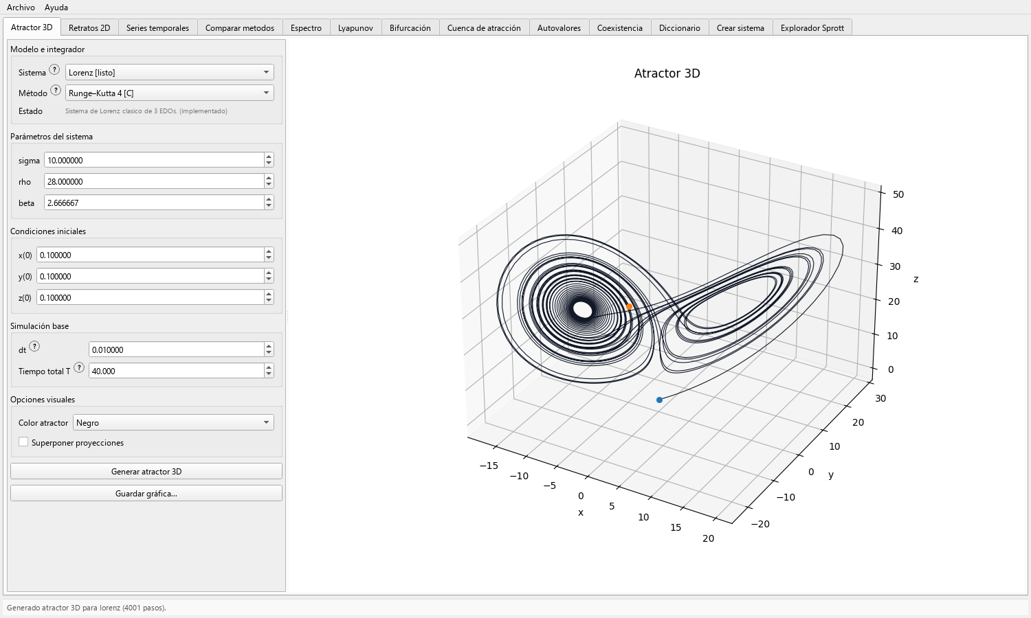
Toolbox Chaos 3D attractor tab showing a Lorenz trajectory
Current interface

3D attractor workspace

Select a registered model, edit parameters and initial conditions, then generate a 3D trajectory.

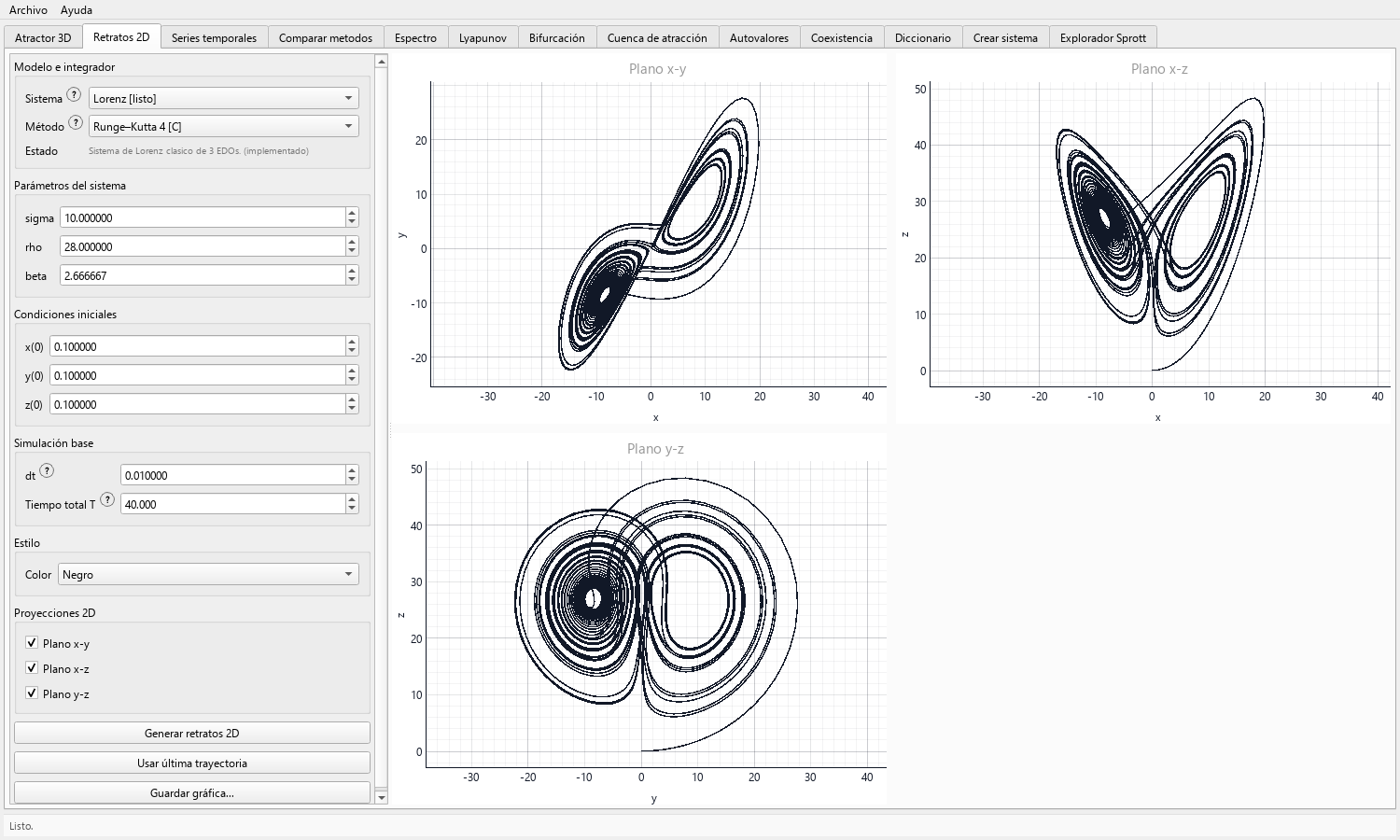
Toolbox Chaos 2D phase portraits tab
Current interface

Phase-portrait workspace

Reuse the last trajectory and compare the xy, xz, and yz projections in one view.

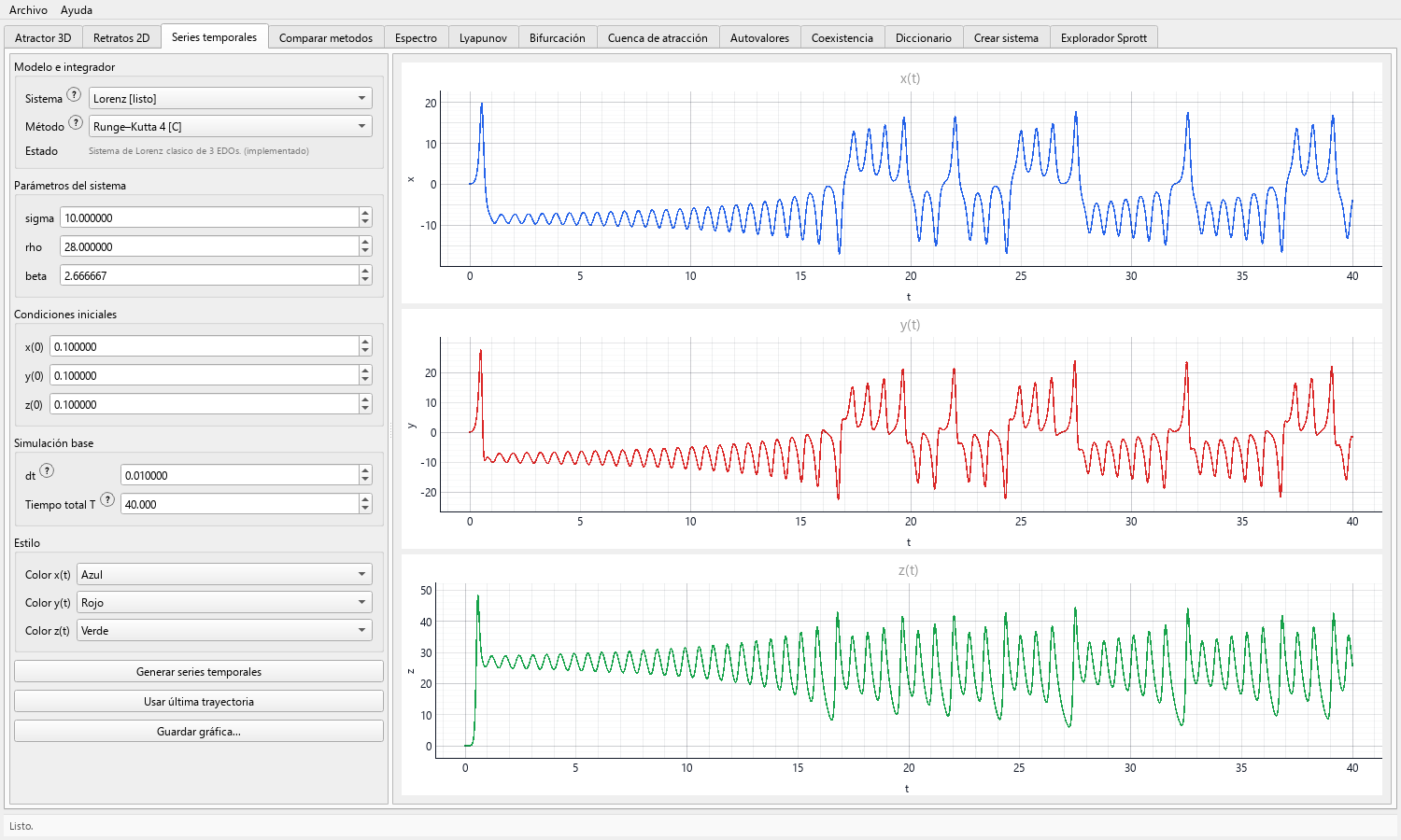
Toolbox Chaos time-series tab
Current interface

Time-series workspace

Inspect each state variable against time while retaining the numerical context of the simulation.

Toolbox Chaos spectral tab showing a Welch power spectral density
Current interface

Welch power spectral density

Choose Welch PSD or an amplitude spectrum, set the transient and frequency range, and preserve physical units.

Toolbox Chaos numerical integrator comparison tab
Current interface

Euler, Heun, and RK4

Overlay three supported integrators to reveal method and time-step sensitivity.

Toolbox Chaos equilibria and eigenvalues tab
Current interface

Equilibria and eigenvalues

List equilibria, plot eigenvalues on the complex plane, and inspect local stability labels.

Toolbox Chaos Lyapunov tab showing the finite-time Lorenz spectrum
Current interface

Lyapunov convergence

Estimate the finite-time Lyapunov spectrum and inspect every convergence curve with its numerical contract.

Toolbox Chaos bifurcation tab showing a Lorenz rho sweep
Current interface

Bifurcation sweep

Sweep a declared parameter and retain Poincare events after a documented transient.

Toolbox Chaos basin tab showing a Lorenz initial-condition classification
Current interface

Basin classification

Classify a grid of initial conditions and overlay the supported equilibria on the sampled plane.

Toolbox Chaos coexistence tab showing the registered Lorenz case
Current interface

Coexistence workspace

Load a referenced case and compare trajectories generated from multiple registered initial conditions.

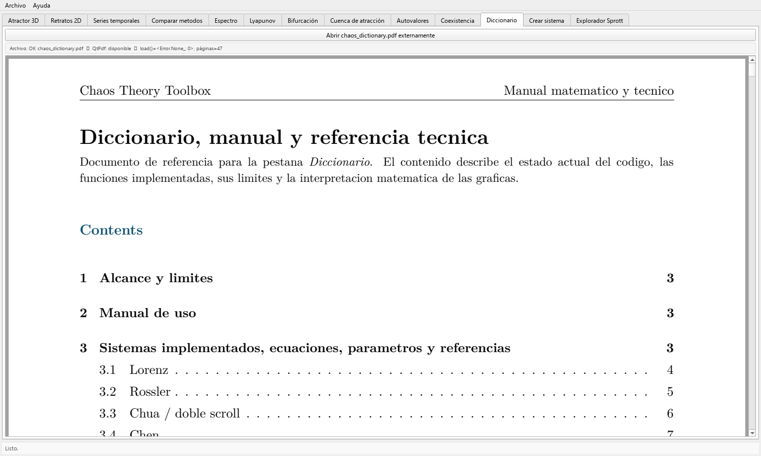
Toolbox Chaos dictionary tab displaying the bundled PDF reference
Current interface

Embedded concept dictionary

Open the bundled mathematical and technical reference from the application.

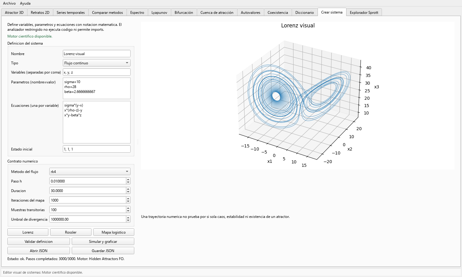
Toolbox Chaos custom-system editor
Current interface

Custom system editor

Define equations and parameters, validate accepted expressions, simulate, and exchange the model as JSON.

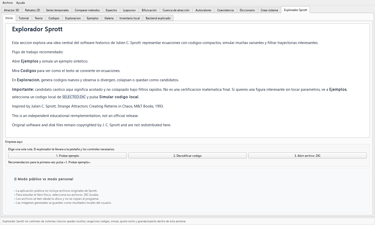
Toolbox Chaos Sprott Explorer home tab
Current interface

Sprott Explorer

Use the tutorial, compact-code decoder, examples, local inventory, gallery, and backend explanation.

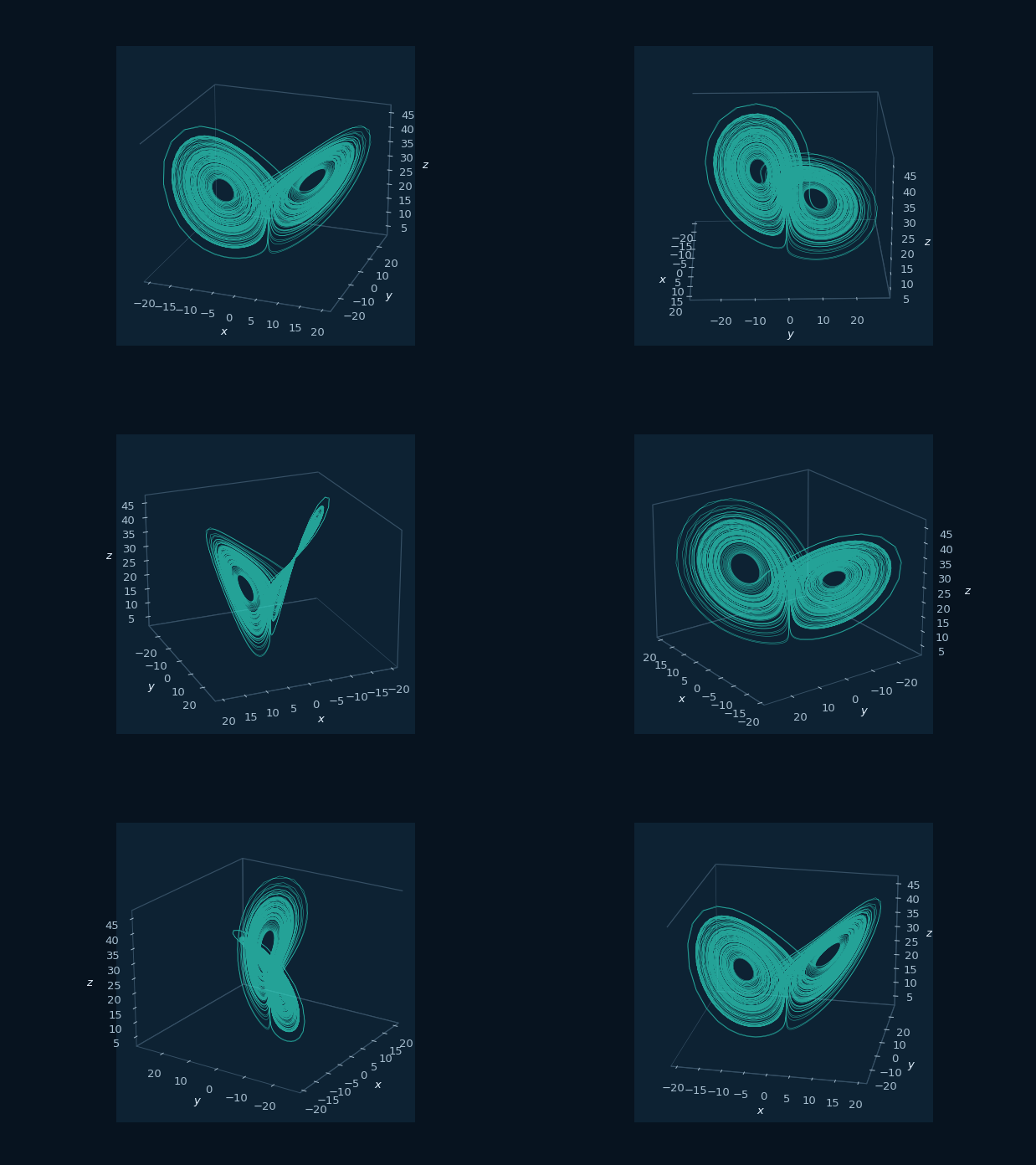
Rotating Lorenz trajectory showing both lobes of the attractor
3D attractors

Lorenz 3D rotation

The rotating view displays the two lobes and the repeated transitions between them.

Side-by-side titleless trajectories for Lorenz, Rossler, and Sprott flows
3D attractors

Geometry across three flows

Lorenz, Rössler, and Sprott trajectories display the folding, rotation, and scale of each flow.

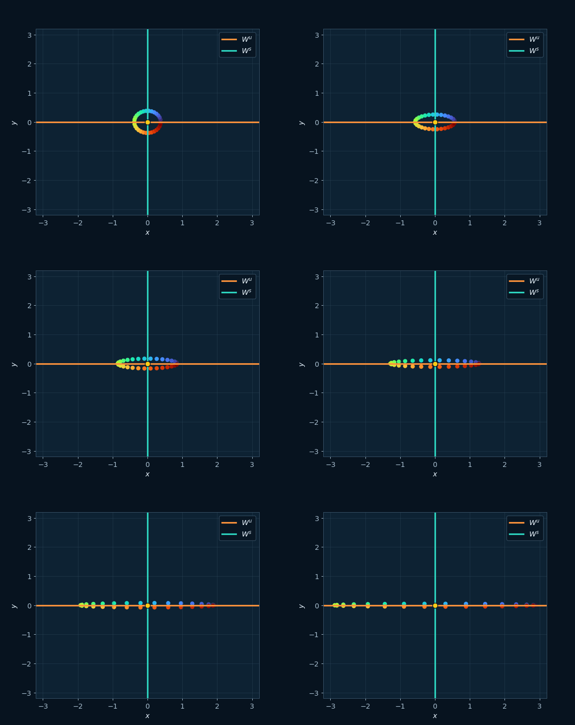
Saddle phase portrait showing stable and unstable invariant manifolds
Phase portraits

Stable and unstable manifolds

The animated saddle separates incoming and outgoing directions around a hyperbolic equilibrium.

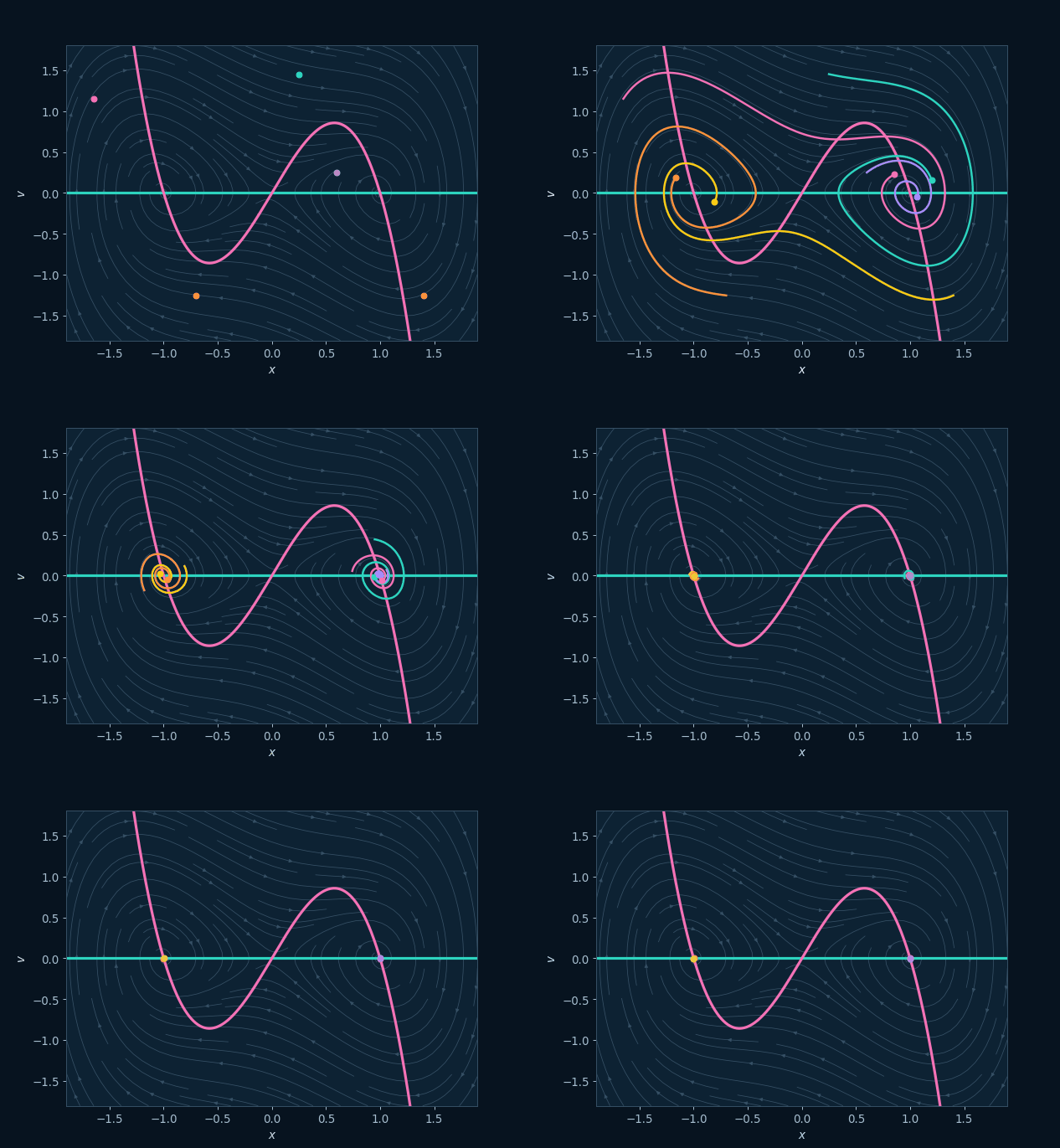
Animated planar flow with nullclines, trajectories, and equilibrium points
Phase portraits

Nullclines and local flow

Motion through the vector field reveals how nullclines partition the plane and locate equilibria.

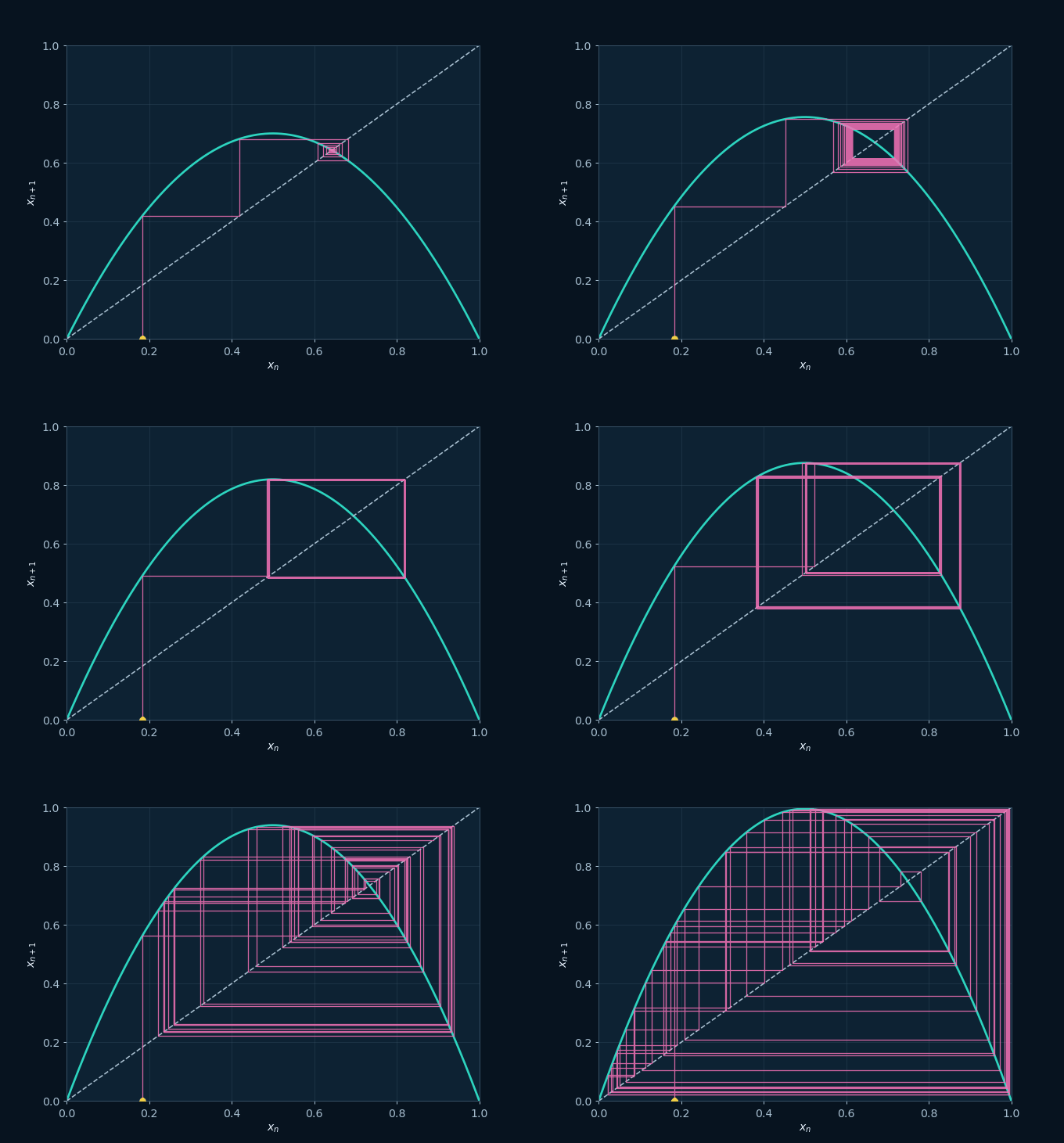
Animated cobweb iteration for the logistic map
Iterated maps

Logistic cobweb

Successive vertical and horizontal segments turn the recurrence into a geometric construction.

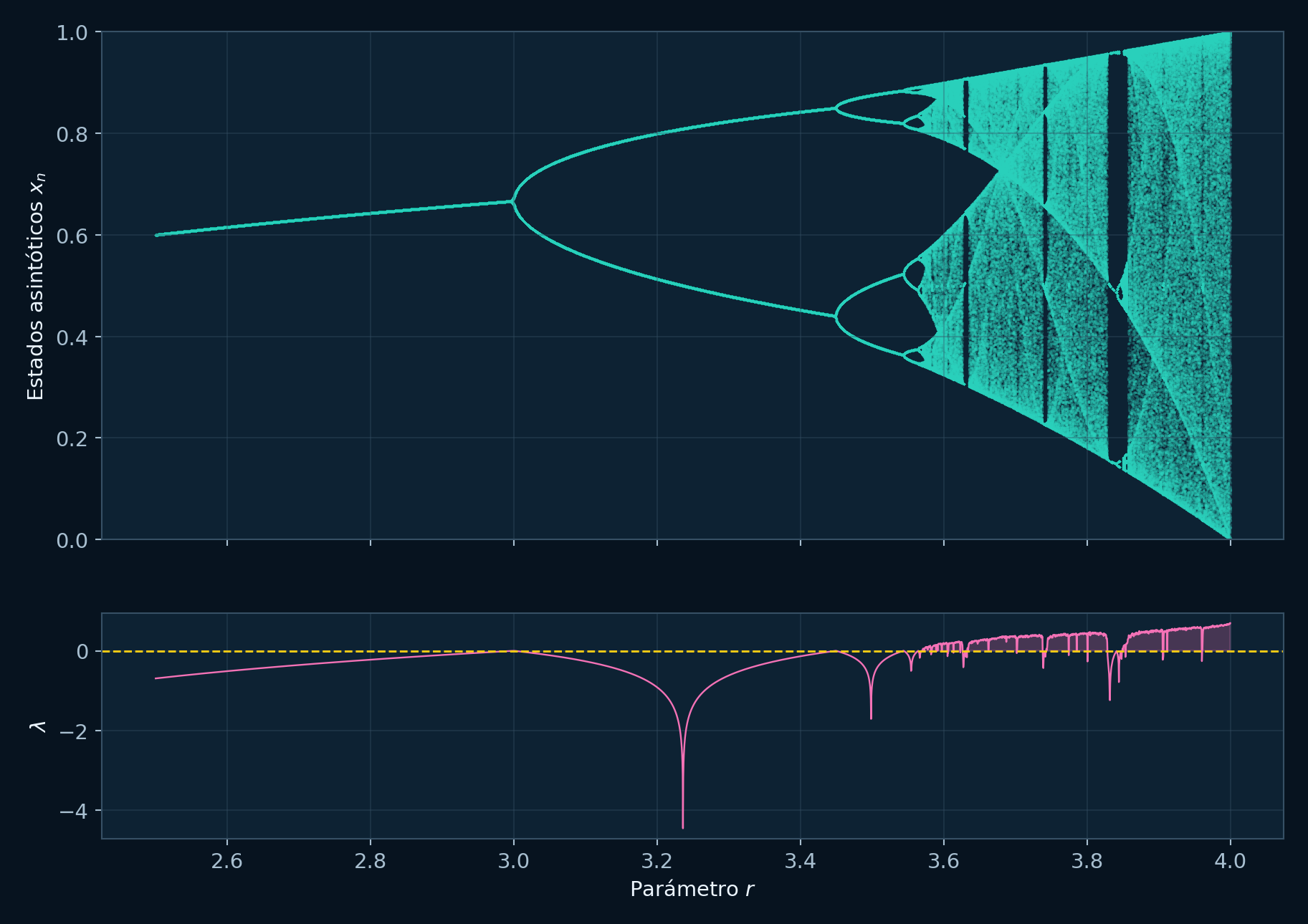
Titleless logistic bifurcation diagram paired with the fixed-point multiplier
Bifurcation

Logistic cascade and stability

Asymptotic states expose period doubling, chaotic bands, periodic windows, and changes in the local multiplier.

Animated Lorenz trajectory accumulating crossings on a Poincare section
Poincare

Lorenz return section

Each accepted crossing turns a continuous 3D flow into a lower-dimensional sequence of returns.

Animated supercritical Hopf bifurcation showing the birth of a limit cycle
Bifurcation

Birth of a Hopf cycle

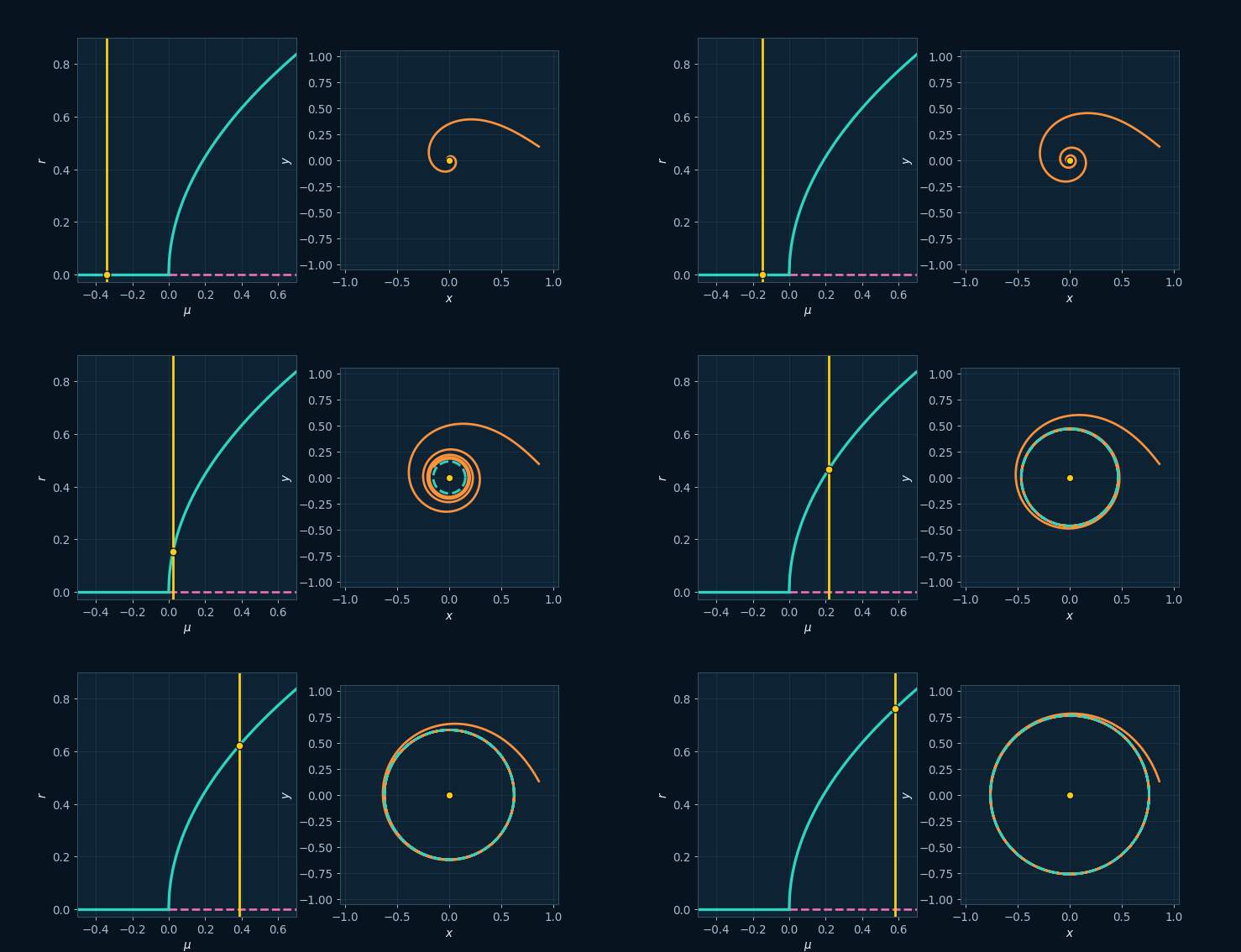
The orbit settles at the equilibrium before the threshold and approaches a growing cycle after it.

Titleless basin map with two destination classes and representative equilibria
Basins

Bistable basin map

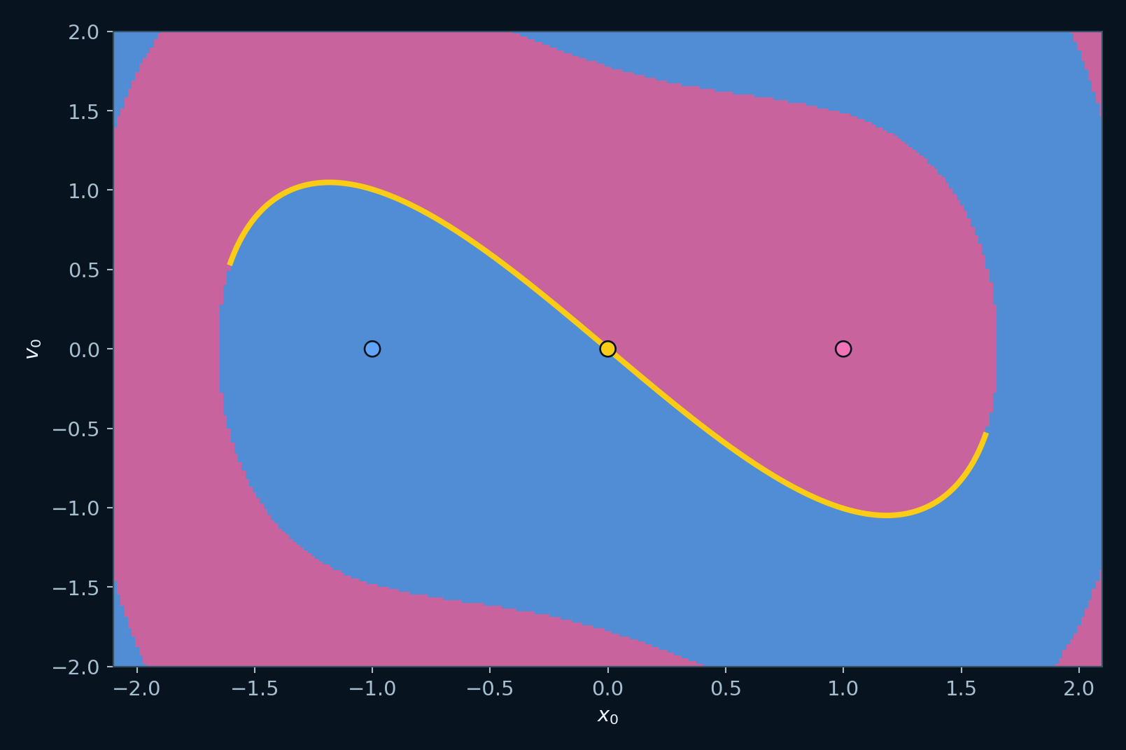
Every initial condition is colored by the destination reached over the declared integration horizon.

Animated refinement of a bistable basin classification grid
Basins

Boundary refinement

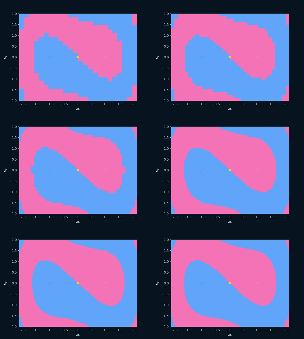
Increasing the initial-condition grid reveals how a smooth-looking boundary can conceal finer structure.

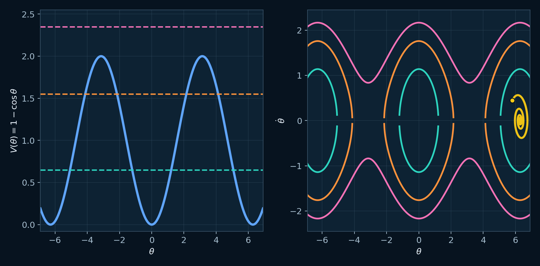
Titleless pendulum potential and phase portrait at several energy levels
Energy and phase

Pendulum energy levels

The potential barriers and phase curves distinguish oscillation, separatrix motion, and rotation.

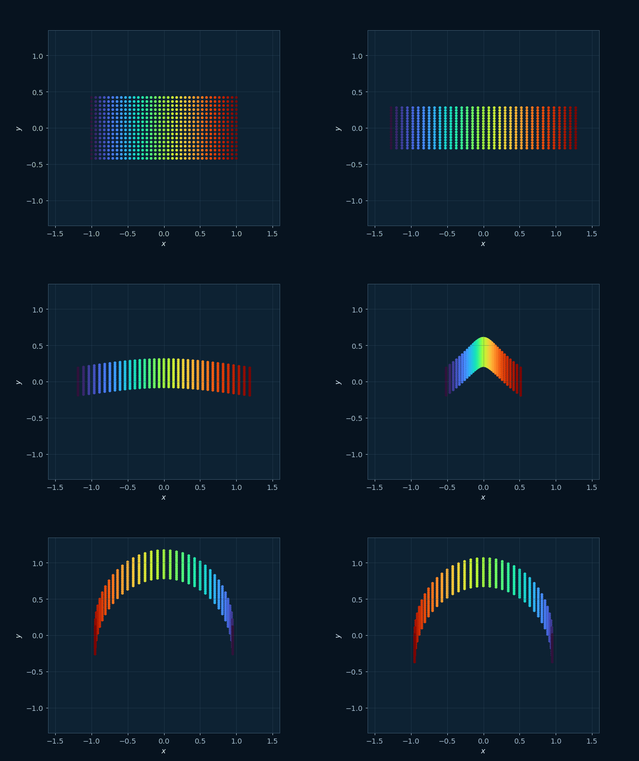
Animated stretching and folding mechanism associated with a chaotic discrete map
Discrete chaos

Stretching and folding

The animation links the geometric horseshoe mechanism with the folded point cloud of an iterated map.

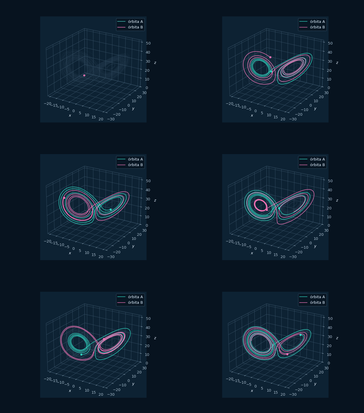
Animated logarithmic separation between two nearby Lorenz trajectories
Lyapunov

Finite-time separation

Nearby Lorenz trajectories separate exponentially at first and later saturate at the attractor scale.

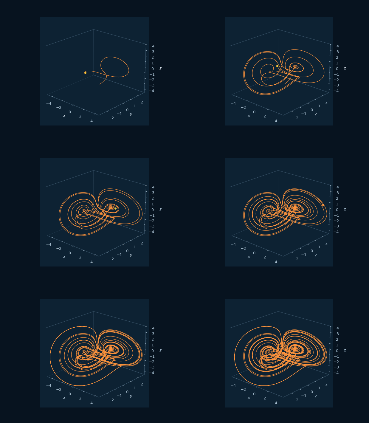
Animated high-contrast orbit of the classical Sprott B flow
Sprott Explorer

Sprott B orbit

The animated trace preserves the thin turns of the compact quadratic flow against the dark canvas.

High-contrast Hénon map showing stretching and folding
Sprott Explorer

Iterated-map geometry

Successive images display the stretching and folding produced by the iterated map.

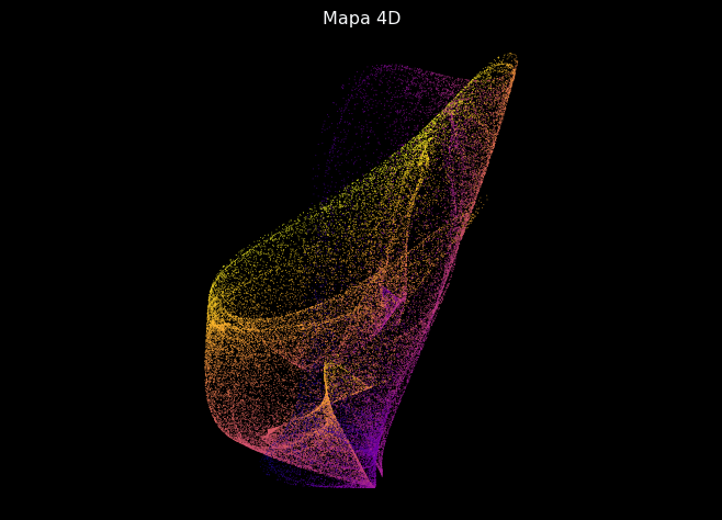
Synthetic 4D Sprott map projected with color
Sprott Explorer

4D projection

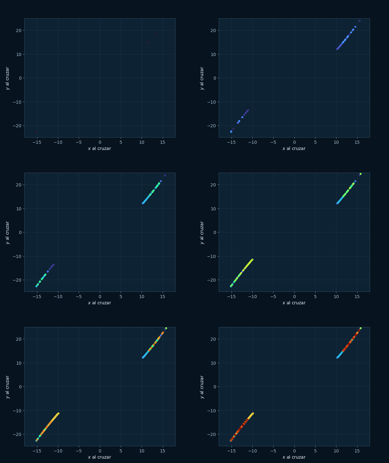
A 4D synthetic map projected with the fourth coordinate in color.

Citing Toolbox Chaos

If you use this software in research, thesis, or academic workflows, cite the archived OSF release.

Maria Fernanda Moreno Lopez. Fyskode Chaotic Systems Toolbox, version 0.1.0. 10.17605/OSF.IO/GQMJR.

Get BibTeX and CFF files ->